Segmentation
This module contains the Segmentation class, responsible for the image segmentation of grain-based materials (rocks, metals, etc.)
Classes
Segmentation of grain-based microstructures |
-
class
grains.segmentation.Segmentation(image_location, save_location=None, interactive_mode=True)[source]¶ Bases:
objectSegmentation of grain-based microstructures
-
original_image¶ Matrix representing the initial, unprocessed image.
- Type
ndarray
-
create_skeleton(boundary_image)[source]¶ Use thinning on the grain boundary image to obtain a single-pixel wide skeleton.
- Parameters
boundary_image (bool ndarray) – A binary image containing the objects to be skeletonized.
- Returns
skeleton (bool ndarray) – Thinned image.
-
filter_image(window_size, image_matrix=None)[source]¶ Median filtering on an image. The median filter is useful in our case as it preserves the important borders (i.e. the grain boundaries).
- Parameters
window_size (int) – Size of the sampling window.
image_matrix (3D ndarray with size 3 in the third dimension, optional) – Input image to be filtered. If not given, the original image is used.
- Returns
filtered_image (3D ndarray with size 3 in the third dimension) – Filtered image, output of the median filter algorithm.
-
find_grain_boundaries(segmented_image)[source]¶ Find the grain boundaries.
- Parameters
segmented_image (ndarray) – Label image, output of a segmentation.
- Returns
boundary (bool ndarray) – A bool ndarray, where True represents a boundary pixel.
-
initial_segmentation(*args)[source]¶ Perform the quick shift superpixel segmentation on an image. The quick shift algorithm is invoked with its default parameters.
- Parameters
*args (3D numpy array with size 3 in the third dimension) – Input image to be segmented. If not given, the original image is used.
- Returns
segment_mask (ndarray) – Label image, output of the quick shift algorithm.
-
merge_clusters(segmented_image, threshold=5)[source]¶ Merge tiny superpixel clusters. Superpixel segmentations result in oversegmented images. Based on graph theoretic tools, similar clusters are merged.
- Parameters
segmented_image (ndarray) – Label image, output of a segmentation.
threshold (float, optional) – Regions connected by edges with smaller weights are combined.
- Returns
merged_superpixels (ndarray) – The new labelled array.
-
save_array(filename, array)[source]¶ Save an image as a numpy array. The array is saved in the standard numpy format, into the directory determined by the save_location attribute.
- Parameters
filename (str) – The array is saved under this name, with extension .npy
array (ndarray) – An image represented as a numpy array.
-
save_image(filename, array, is_label_image=False)[source]¶ Save an image as a numpy array. The array is saved in the standard numpy format, into the directory determined by the save_location attribute.
- Parameters
filename (str) – The array is saved under this name, with extension .npy
array (ndarray) – An image represented as a numpy array.
is_label_image (bool) – True if the array represents a labeled image.
-
watershed_segmentation(skeleton)[source]¶ Watershed segmentation of a granular microstructure. Uses the watershed transform to label non-overlapping grains in a cellular microstructure given by the grain boundaries.
- Parameters
skeleton (bool ndarray) – A binary image, the skeletonized grain boundaries.
- Returns
segmented (ndarray) – Label image, output of the watershed segmentation.
-
Gala
A trimmed version of the Gala project (https://github.com/janelia-flyem/gala) with some additions (new function, added documentation for the existing ones). Gala is licensed by the Janelia Farm License: http://janelia-flyem.github.io/janelia_farm_license.html
Copyright 2012 HHMI. All rights reserved.
Redistribution and use in source and binary forms, with or without modification, are permitted provided that the following conditions are met:
Redistributions of source code must retain the above copyright notice, this list of conditions and the following disclaimer. Redistributions in binary form must reproduce the above copyright notice, this list of conditions and the following disclaimer in the documentation and/or other materials provided with the distribution.
Neither the name of HHMI nor the names of its contributors may be used to endorse or promote products derived from this software without specific prior written permission.
THIS SOFTWARE IS PROVIDED BY THE COPYRIGHT HOLDERS AND CONTRIBUTORS “AS IS” AND ANY EXPRESS OR IMPLIED WARRANTIES, INCLUDING, BUT NOT LIMITED TO, THE IMPLIED WARRANTIES OF MERCHANTABILITY AND FITNESS FOR A PARTICULAR PURPOSE ARE DISCLAIMED. IN NO EVENT SHALL THE COPYRIGHT OWNER OR CONTRIBUTORS BE LIABLE FOR ANY DIRECT, INDIRECT, INCIDENTAL, SPECIAL, EXEMPLARY, OR CONSEQUENTIAL DAMAGES (INCLUDING, BUT NOT LIMITED TO, PROCUREMENT OF SUBSTITUTE GOODS OR SERVICES; LOSS OF USE, DATA, OR PROFITS; OR BUSINESS INTERRUPTION) HOWEVER CAUSED AND ON ANY THEORY OF LIABILITY, WHETHER IN CONTRACT, STRICT LIABILITY, OR TORT (INCLUDING NEGLIGENCE OR OTHERWISE) ARISING IN ANY WAY OUT OF THE USE OF THIS SOFTWARE, EVEN IF ADVISED OF THE POSSIBILITY OF SUCH DAMAGE.
Functions
|
Extended-minima transform. |
|
Suppress all minima that are shallower than thresh. |
|
Suppress all minima that are shallower than thresh. |
|
Perform morphological reconstruction of the marker into the mask. |
|
Find the regional minima in an ndarray. |
|
-
grains.gala_light.hminima(a, thresh)[source]¶ Suppress all minima that are shallower than thresh.
- Parameters
a (array) – The input array on which to perform hminima.
thresh (float) – Any local minima shallower than this will be flattened.
- Returns
out (array) – A copy of the input array with shallow minima suppressed.
-
grains.gala_light.imextendedmin(image, h, connectivity=1)[source]¶ Extended-minima transform. The extended minima transform is the regional minima of the h-minima transform. The implementation follows the MATLAB function under the same name.
- Parameters
image (ndarray) – The input array on which to perform imextendedmin.
h (float) – Any local minima shallower than this will be flattened.
connectivity (int, optional) – Determines which elements are considered as neighbors of the central element. Elements up to a squared distance of connectivity from the center are considered neighbors. If connectivity=1, no diagonal elements are neighbors.
- Returns
bool ndarray – True at places of the extended minima.
-
grains.gala_light.imhmin(a, thresh)¶ Suppress all minima that are shallower than thresh.
- Parameters
a (array) – The input array on which to perform hminima.
thresh (float) – Any local minima shallower than this will be flattened.
- Returns
out (array) – A copy of the input array with shallow minima suppressed.
-
grains.gala_light.morphological_reconstruction(marker, mask, connectivity=1)[source]¶ Perform morphological reconstruction of the marker into the mask.
See the Matlab image processing toolbox documentation for details: http://www.mathworks.com/help/toolbox/images/f18-16264.html
Analysis
This module contains the Analysis class, responsible for the analysis of segmented grain-based microstructures.
All the examples assume that the modules numpy and matplotlib.pyplot were imported as np and plt, respectively.
Functions
|
Determines the maximum Feret diameter. |
|
Plots relevant region properties into a single figure. |
|
Plots the distribution of a given grain characteristic. |
|
Displays a labeled image. |
|
Skeleton of a labeled image. |
|
Thickens a skeleton by morphological dilation. |
|
Changes parts of a labeled image to a given value. |
-
class
grains.analysis.Analysis(label_image, interactive_mode=False)[source]¶ Bases:
objectAnalysis of grain assemblies.
-
original_image¶ Matrix representing the initial, unprocessed image.
- Type
ndarray
-
compute_properties()[source]¶ Determines relevant properties of the grains. The area of each grain is determined in the units previously given in the set_scale method.
- Parameters
window_size (int) – Size of the sampling window.
image_matrix (3D ndarray with size 3 in the third dimension, optional) – Input image to be filtered. If not given, the original image is used.
- Returns
filtered_image (3D ndarray with size 3 in the third dimension) – Filtered image, output of the median filter algorithm.
-
set_scale(pixel_per_unit=1)[source]¶ Defines a scale for performing computations in that unit. Image measures (area, diameter, etc.) are performed on a matrix corresponding to a label image. Therefore, the result of all the computations are obtained in pixel units. It is often of interest to access the results in physical units (mm, cm, inch, etc.). Manually converting pixels, pixel squares, etc. to pyhsical units, physical unit sqaures, etc. are tedious and error prone. Once the conversion between a pixel and a physical unit is given, all the subsequent calculations are performed in the desired physical unit.
- Parameters
pixel_per_unit (float or int or scalar ndarray, optional) – Number of pixels contained in a certain unit. The default is 1, in which case all measurements are performed in pixel units.
- Returns
None.
-
show_grains(grain_property=None)[source]¶ Display the grains, optionally with a property superposed.
- Parameters
- grain_property ({None, ‘area’, ‘centroid’, ‘coordinate’,) – ‘equivalent_diameter’, ‘feret_diameter’, ‘label’}
optional
If not None, the selected property is shown on the grain as text.
- Returns
None.
-
show_properties(gui=False)[source]¶ Displays previously computed properties of the grains
- Parameters
gui (bool, optional) – If true, the grain properties are shown in a GUI. If false, they are printed to stdout. The default is False. The GUI requires the dfgui modul, which can be obtained from https://github.com/bluenote10/PandasDataFrameGUI
- Returns
None.
-
-
grains.analysis.feret_diameter(prop)[source]¶ Determines the maximum Feret diameter.
- Parameters
prop (RegionProperties) – Describes a labeled region.
- Returns
max_feret_diameter (float) – Maximum Feret diameter of the region.
See also
skimage.measure.regionprops()Measure properties of labeled image regions
Examples
>>> import numpy as np
>>> from skimage.measure import regionprops
>>> image = np.ones((2,2), dtype=np.int8)
>>> prop = regionprops(image)[0]
>>> feret_diameter(prop)
2.23606797749979
-
grains.analysis.label_image_apply_mask(label_image, mask, value)[source]¶ Changes parts of a labeled image to a given value.
Convenience function, equivalent to
label_image[mask] = valuebut the original arraylabel_imageis not overwritten.- Parameters
label_image (ndarray) – Labeled input image, represented as a 2D numpy array of positive integers.
mask (ndarray) – Boolean array of the same size as
label_image, marking the pixels that will be replaced byvalue.value (int) – The masked pixels are replaced by this value.
- Returns
ndarray – Copy of the input image, its selected pixels being replaced by the given value.
-
grains.analysis.label_image_skeleton(label_image)[source]¶ Skeleton of a labeled image.
The skeleton of a labeled image is a single-pixel wide network that separates the labeled regions.
- Parameters
label_image (ndarray) – Labeled input image, represented as a 2D numpy array of positive integers.
- Returns
ndarray – A 2D bool numpy array having the same size as
label_image, where True represents the skeleton pixels.
See also
-
grains.analysis.plot_grain_characteristic(characteristic, centers, interpolation='linear', grid_size=(100, 100), **kwargs)[source]¶ Plots the distribution of a given grain characteristic.
One way to gain insight into a grain assembly is to plot the distribution of a certain grain property in the domain the grains occupy. In this function, for each grain, and arbitrary (scalar) quantity is associated to the center of the grain. In case of n grains, n data points span the interpolant and the given characteristic is interpolated on a grid of the AABB of the grain centers.
- Parameters
characteristic (ndarray) – Characteristic property, the distribution of which is sought. A 1D numpy array.
centers (ndarray) – 2D numpy array with 2 columns, each row corresponding to a grain, and the two columns giving the Cartesian coordinates of the grain center.
interpolation ({‘nearest’, ‘linear’, ‘cubic’}, optional) – Type of the interpolation for creating the distribution. The default is ‘linear’.
grid_size (tuple of int, optional) – 2-tuple, the size of the grid on which the data is interpolated. The default is (100, 100).
- Other Parameters
center_marker (str, optional) – Marker indicating the center of the grains. The default is ‘P’. For a list of supported markers, see the documentation. If you do not want the centers to be shown, choose ‘none’.
show_axis (bool, optional) – If True, the axes are displayed. The default is False.
- Returns
None
See also
Notes
This function knows nothing about how the center of a grain is determined and what characteristic features a grain has. It only performs interpolation and visualization, hence decoupling the plotting from the actual representation of grains and their characteristics. For instance, a grain can be represented as a spline surface, as a polygon, as an assembly of primitives (often triangles), as pixels, just to mention some typical scenarios. Calculating the center of a grain depends on the grain representation at hand. Similarly, one can imagine various grain characteristics, such as area, diameter, Young modulus.
Examples
Assume that the grain centers are sampled from a uniformly random distribution on the unit square.
>>> n_data = 100
>>> points = np.random.random((n_data, 2))
The quantity we want to plot has a parabolic distribution with respect to the position of the grain centers.
>>> func = lambda x, y: 1 - (x-0.5)**2 - (y-0.5)**2
>>> plot_grain_characteristic(func(points[:, 0], points[:, 1]), points, center_marker='*')
>>> plt.show()
-
grains.analysis.plot_prop(prop, pixel_per_unit=1, show_axis=True)[source]¶ Plots relevant region properties into a single figure. Four subfigures are created, giving the region’s
image, its area and its center
filled image, its area
bounding box, its area
convex image, its area
- Parameters
prop (RegionProperties) – Describes a labeled region.
pixel_per_unit (float or int, optional) – Number of pixels contained in a certain unit. The default is 1, in which case all measurements are performed in pixel units.
- Returns
fig (matplotlib.figure.Figure) – The figure object is returned in case further manipulations are necessary.
-
grains.analysis.show_label_image(label_image, alpha=1)[source]¶ Displays a labeled image.
A random color is associated with each labeled region. If boundary pixels are present in the image, they are plotted in black.
- Parameters
label_image (ndarray) – Labeled input image, represented as a 2D numpy array of non-negative integers. The label 0 is assumed to denote a boundary pixel.
alpha (float, optional) – Opacity of colorized labels. Must be within [0, 1].
- Returns
None
-
grains.analysis.thicken_skeleton(skeleton, thickness)[source]¶ Thickens a skeleton by morphological dilation.
- Parameters
skeleton (ndarray) – Skeleton of a binary image, represented as a bool 2D numpy array.
thickness (int) – Thickness of the resulting boundaries.
- Returns
ndarray – A 2D bool numpy array, where True represents the thickened skeleton.
See also
-
grains.analysis.truecolor2label(color_image)[source]¶ Truecolor image into labeled image.
It is often the case that you need to deal with a labeled image that was saved as a truecolor image (e.g. RGB). A labeled region is then the set of pixels with the same colors.
- Parameters
color_image (ndarray) – 3D array, the first two dimensions corresponding to the image pixels, the third one for the channels (e.g. RGB, HSV, CMYK, etc.).
- Returns
ndarray – Labeled image, represented as a 2D numpy array of non-negative integers.
Meshing
Classes
-
class
grains.meshing.OOF2[source]¶ Bases:
object-
create_material(name)[source]¶ - Parameters
name (TYPE) – DESCRIPTION.
- Raises
Exception – DESCRIPTION.
- Returns
None.
-
create_microstructure(name=None)[source]¶ Creates a microstructure from an image.
- Parameters
name (str, optional) – Path to the image on which the microstucture is created, file extension included. If not given, the microstructure is given the same name as the input image.
- Raises
Exception – DESCRIPTION.
- Returns
None.
-
load_pixelgroups(microstructure_file)[source]¶ - Parameters
microstructure_file (str) – DESCRIPTION.
- Returns
None.
-
materials2groups(materials, groups=None)[source]¶ - Parameters
materials (list of str) – DESCRIPTION.
groups (list of int, optional) – DESCRIPTION. The default is None.
- Returns
None.
-
script= []
-
-
class
grains.meshing.QuadSkeletonGeometry(leftright_periodicity=False, topbottom_periodicity=False)[source]
-
class
grains.meshing.SkeletonGeometry(leftright_periodicity, topbottom_periodicity)[source]¶ Bases:
abc.ABC
-
class
grains.meshing.TriSkeletonGeometry(leftright_periodicity=False, topbottom_periodicity=False, arrangement='conservative')[source]
-
grains.meshing.nt¶ alias of
grains.meshing.modules
CAD
MED
Extracting and processing meshes from .med files. The functions were tested on the MEDCoupling API, version 9.4.0.
Todo
Support renumbering (https://docs.salome-platform.org/latest/dev/MEDCoupling/user/html/data_optimization.html).
Getting help:
This module relies on the Python interface of MEDCoupling. Click here for the latest documentation.
User’s manual for the Python interface
To know more about the MED file format, which is a specialization of HDF5, see the documentation. For a discussion on the relation between the MED format and the APIS, see this page and that one.
The definitions, such as group, used in this module are from the development guide.
A (mostly English) tutorial for the Python interface to MEDCoupling is also useful. Particularly interesting are the mesh manipulation examples
Main page of the documentation
Functions
Reads a mesh file in .med format. |
|
Obtains the nodes and the node groups of a mesh. |
|
Obtains the elements for each group of a mesh. |
-
grains.med.get_elements(mesh, numbering='global')[source]¶ Obtains the elements for each group of a mesh.
Elements of the same dimension as the mesh are collected (e.g. faces for a 2D mesh).
Todo
put those elements that do not belong to any group into an automatically created group
Todo
support ordering elements in alphabetical order
Todo
implement the ‘global’ strategy
- Parameters
mesh (MEDFileUMesh) – Unstructured mesh.
numbering ({‘global’}, optional) –
- Determines how to allocate element numbers in the mesh.
‘global’: numbers the elements without taking into account which group they belong to. Use this strategy if you are not sure whether an element belongs to more than one group. ‘group’: numbers the elements group-wise. This is much faster than the ‘global’ strategy, but use this option if you are sure that the groups of the mesh do not contain common elements.
The default is ‘global’.
- Returns
elements (ndarray) – Element-node connectivities in a 2D numpy array, in which each row corresponds to an element and the columns are the nodes of the elements. It is assumed that all the elements have the same number of nodes.
element_groups (dict) – The keys in the dictionary are the element group names, while the values are list of integers, giving the elements that belong to the particular group.
Warning
Currently, elements that do not fit into any groups are discarded.
See also
get_nodes(),change_node_numbering()Notes
The element-node connectivities are read from the mesh. If you want to change the ordering of the nodes, use the
change_node_numbering()function.Both this and the
get_nodes()function relies on getGroupsOnSpecifiedLev to obtain the groups based on a parameter, called meshDimRelToMaxExt. This parameter designates the relative dimension of the mesh entities whose IDs are required. If it is 1, it denotes the nodes. If 0, entities of the same dimension as the mesh are meant (e.g. group of volumes for a 3D mesh, or group of faces for a 2D mesh). When -1, entities of spatial dimension immediately below that of the mesh are collected (e.g. group of faces for a 3D mesh, or group of edges for a 2D mesh). For -2, entities of two dimensions below that of the mesh are fetched (e.g. group of edges for a 3D mesh).
-
grains.med.get_nodes(mesh)[source]¶ Obtains the nodes and the node groups of a mesh.
- Parameters
mesh (MEDFileUMesh) – Unstructured mesh.
- Returns
nodes (ndarray) – 2D numpy array with 2 columns, each row corresponding to a node, and the two columns giving the Cartesian coordinates of the nodes.
node_groups (dict) – The keys in the dictionary are the node group names, while the values are list of integers, giving the nodes that belong to the particular group.
See also
-
grains.med.read_mesh(filename)[source]¶ Reads a mesh file in .med format. Only one mesh, the first one, is supported. However, that mesh can contain groups.
- Parameters
filename (str) – Path to the mesh file.
- Returns
MEDFileUMesh – Represents an unstructured mesh. For details, see the manual on https://docs.salome-platform.org/latest/dev/MEDCoupling/developer/classMEDCoupling_1_1MEDFileUMesh.html
Salome
The documentation generated from this file is available on https://cristalx.readthedocs.io/en/latest/api.html#module-grains.salome.
The aim of this module is to manage geometry and mesh operations on
two-dimensional microstructures that tessellate a domain. This has the important consequence that
the domain is assumed to consist of non-overlapping shapes that cover it. After generating a
conforming mesh, each element belongs to a single group and no element exists outside the
group. More precisely, elements that do not belong to any group are not taken into account by the
Mesh class. They can still be accessed by the functions of Salome, but the use of such
lower-level abstractions is against the philosophy of encapsulation this module provides.
The non-goals of this module include everything not related to the tessellation nature of 2D microstructures. The emphasis is on readability and not on speed.
This file can be used either as a module or as a script.
Using as a module
Developers, implementing new features, will use salome.py as a Python module. Although this
module is part of the grains package in the CristalX project, it does not rely on the other modules of
grains. This ensures that it can be used standalone and run as a script in the Salome environment. It only uses language constructs available in Python 3.6,
and external packages shipped with Salome 9.4.0 onwards. To enable debugging, code completion
and other useful development methods, consult with the documentation on …
Most classes contain a protected variable that holds the underlying Salome object. Unless you
debug, it is not necessary to directly deal with Salome objects programmatically.
Using as a script
When salome.py is run as a script, the contents in the if __name__ == "__main__": block
is executed. Edit it to suit your needs. Similarly to the case when used as a module, the script can only be run from Salome’s own Python interpreter: either from
the shell or from the GUI. To run it from the shell (including the GUI’s built-in Python command
prompt), type
exec(open("<path_to_CristalX>/grains/salome.py", "rb").read())
You can also execute the script from the GUI by clicking on …
Classes
Represents the geometrical entities of a two-dimensional tessellated domain. |
|
Closed part of a plane. |
|
A shape corresponding to a curve, and bounded by a vertex at each extremity. |
|
An edge between two faces. |
|
Performs mesh manipulations on a tessellated geometry. |
|
Mesh on a face, part of the whole mesh. |
|
Mesh on an interface, part of the whole mesh. |
|
Constructs zero-thickness elements along the interfaces. |
|
Using GUI-related functionalities in Salome. |
-
class
grains.salome.CohesiveZone(mesh)[source]¶ Bases:
objectConstructs zero-thickness elements along the interfaces.
- Parameters
mesh (Mesh) – Mesh into which the cohesive elements will be inserted.
-
_affected_elements(interface_mesh)[source]¶ Face elements whose nodes must be renumbered when duplicating an interface mesh.
- Parameters
interface_mesh (InterfaceMesh) – The original interface mesh that will be duplicated.
- Returns
elements (set) – Elements of the mesh that require node renumbering.
See also
-
_correct_junction_nodes()[source]¶ Post-processing to handle inconsistent interface nodes at the junctions.
The interface-wise creation of new edge elements in
_affected_elements()may result in edge element nodes that do not connect the opposite face element nodes on the two sides of the interface. This function checks the edge element nodes at the junctions and renumbers them so that they hold the same label as the face element nodes they connect to.- Returns
None.
-
_enrich_interfaces()[source]¶ Inserts new interface elements and nodes into the mesh.
Although Salome has built-in functionality for duplicating nodes and creating elements, even accessible from the GUI with Modification -> Transformation -> Duplicate Nodes and/or Elements, it does not work with multiple intersecting interfaces or for closed interfaces. The reason is that the first step of the two-step procedure Salome performs fails in such situations. Therefore, this method uses a modified algorithm for the first step, and then calls the second step. These steps are the following:
1. Find the elements (called affected elements) in the mesh whose node numbers need to be changed due to the topological changes in the mesh caused by the introduction of new nodes.
2. The affected elements are fed to an existing function in Salome, which returns the 1D elements it creates from the duplicated nodes. The new interface mesh is stored in the
CohesiveZoneobject.- Returns
None.
-
_generate_cohesive_element(bottom_element, top_element)[source]¶ Creates a zero-thickness quadrilateral element.
- Parameters
bottom_element (int) – Edge element that will form the bottom edge of the cohesive element.
top_element (int) – Edge element that will form the top edge of the cohesive element. It is assumed that the top element geometrically overlaps with the bottom element.
- Returns
list of int – The four nodes of the cohesive element, numbered counter-clockwise. The node ordering adheres to the node numbering in Abaqus.
-
create_cohesive_elements()[source]¶ Creates zero-thickness quadrilateral elements along the interfaces.
It is necessary that the mesh has already been decoupled along the interfaces by the
decouple_faces()method. That method introduced duplicated nodes and edge elements along the interfaces. The purpose of this method is to tie each interface (edge) element to its corresponding duplicate in order to form a four-noded zero-thickness element, referred to as cohesive element. The bottom edge of the new cohesive element corresponds to the original edge element, while its top edge is formed by the duplicated interface edge element.- Returns
cohesive_elements (list) – List of nodes that form the cohesive elements. The node numbering follows the node ordering of Salome, which is the same as the node ordering in Abaqus.
-
decouple_faces()[source]¶ Decouples the face meshes along the interfaces.
The algorithm consists of two main steps. First, new interface meshes are created that overlap with the existing ones and contain independent nodes and interface elements. In the same step, the incident face mesh nodes are updated to reflect the topological changes. However, in this method, extra nodes are introduced at the junctions, leading to a kinematic inconsistency. Therefore, the extraneous interface mesh nodes are renumbered in the second step of the algorithm.
- Returns
None.
See also
-
class
grains.salome.Edge(edge, name)[source]¶ Bases:
objectA shape corresponding to a curve, and bounded by a vertex at each extremity.
An
Edgeknows about theFaceit is part of, and the faces neighboring it.- Parameters
edge (GEOM_Object of shape type ‘EDGE’) – The main Salome object wrapped by this class.
name (str) – Name of the edge.
See also
-
class
grains.salome.Face(face, name)[source]¶ Bases:
objectClosed part of a plane.
A
Faceknows about theEdgeobjects that bound it.- Parameters
face (GEOM_Object of shape type ‘FACE’) – The main Salome object wrapped by this class.
name (str) – Name of the face.
See also
-
class
grains.salome.FaceMesh(face_mesh, name, on_face)[source]¶ Bases:
objectMesh on a face, part of the whole mesh.
- Parameters
face_mesh (smeshBuilder.Mesh.GroupOnGeom) – The main Salome object wrapped by this class.
name (str) – Name of the face mesh.
on_face (Face) – Geometrical face on which this mesh exists.
-
elements()[source]¶ Retrieves the elements of the face mesh.
- Returns
list of int – Elements belonging to the face mesh.
See also
-
class
grains.salome.GUI[source]¶ Bases:
objectUsing GUI-related functionalities in Salome.
Notes
A part of Salome’s GUI is exposed to Python. To get an idea of what is available, see https://docs.salome-platform.org/latest/gui/GUI/text_user_interface.html
-
exception
SalomeNoDesktop[source]¶ Bases:
ExceptionRaised when Salome is run without desktop, but a desktop functionality is invoked.
-
classmethod
_get_component(obj)[source]¶ Determines the component of an object.
This function maps a class of this module to the Salome module the class uses. For instance, class
Faceis mapped to ‘GEOM’.- Parameters
obj – Any object for which the component name is looked for.
- Returns
str or None – The name of the component the object belongs to. If an object of an unsupported class is given, None is returned. For the list of supported classes, see the
component_mapmember ofGUIclass.
See also
-
static
assert_salome_desktop()[source]¶ Checks if Salome’s GUI is available, and raises an exception if it is not.
This function acts as a helper function when relying on Salome’s GUI.
- Raises
SalomeNoDesktop – If Salome’s GUI is not available.
-
component_map= {<class 'grains.salome.Geometry'>: 'GEOM', <class 'grains.salome.Face'>: 'GEOM', <class 'grains.salome.Edge'>: 'GEOM', <class 'grains.salome.Interface'>: 'GEOM', <class 'grains.salome.Mesh'>: 'SMESH', <class 'grains.salome.FaceMesh'>: 'SMESH', <class 'grains.salome.InterfaceMesh'>: 'SMESH'}
-
static
has_desktop()[source]¶ Indicates if the Salome GUI is running.
- Returns
bool – True if Salome’s GUI is available, False otherwise.
-
classmethod
show(obj, show_only=False)[source]¶ Shows objects in Salome’s GUI.
Todo
Support list of objects.
- Parameters
obj (iterable) – The object(s) to be shown in Salome. Objects of the following classes are supported: Geometry, Face, Edge, Interface, Mesh, FaceMesh, InterfaceMesh.
show_only (bool, optional) – If True, the other objects are hidden. The default value is False.
- Returns
None
- Raises
SalomeNoDesktop – If Salome’s GUI is not available.
TypeError – If
objis not an object that can be displayed.ValueError – If the given object does not exist in the Salome study.
Examples
For example, you can display an interface mesh and a face mesh by calling
GUI.show([interface_mesh, face_mesh])
where
interface_meshandface_meshareInterfaceMeshandFaceMeshobjects respectively. This way of using the show method provides great flexibility as different types of objects can be handled at the same time.
-
exception
-
class
grains.salome.Geometry(name='microstructure')[source]¶ Bases:
objectRepresents the geometrical entities of a two-dimensional tessellated domain.
A
Geometryobject knows about the faces that tessellate the domain, and about the edges and interfaces that separate the faces.- Parameters
name (str, optional) – Name of the geometry.
-
_find_overlapping_edges()[source]¶ Finds edges that are on top of each other.
Overlapping edges have the same length. Although its converse is not true in general, we will assume so. This part of the algorithm (i.e. deciding the overlapping edges) can later be refined.
- Returns
overlapping_edges (list) – Each member of the list contains a list of (supposedly) two Edge objects.
See also
-
static
_has_smaller_ID(edges)[source]¶ Selects the edge with a smaller ID.
When generating mesh with the NETGEN plugin of Salome, if several edges overlap, only the edge with the smallest ID holds a mesh. The purpose of this function is to find the edge with the smaller ID out of two overlapping edges.
- Parameters
edges (list of Edge) – List of two Edge objects.
- Returns
Edge – Either the first or the second element of the input list, depending on which of them has a smaller ID.
See also
Notes
For a detailed discussion on this highly important issue, see the corresponding forum thread.
-
create_interfaces()[source]¶ Constructs unique interfaces that separate the faces.
Based on the edges (obtained by exploding the mesh), interfaces are created. Interfaces are unique separators of two neighboring faces. In other words,
if the edge is a boundary edge, no interface is created,
two neighboring faces have two overlapping edges, of which one is defined to be an interface.
It is assumed that the edges and faces of the geometry have already been obtained.
- Returns
None.
See also
-
extract_edges()[source]¶ Decomposes each face into edges.
This method must be called after the
extract_faces()method, otherwise it has no effect.- Returns
None.
See also
-
class
grains.salome.Interface(edge, name, neighboring_faces)[source]¶ Bases:
objectAn edge between two faces.
Similar to an
Edge, but two neighboringFaceobjects share a commonInterface. AnInterfaceknows about the two faces that it separates.- Parameters
edge (GEOM_Object of shape type ‘EDGE’) – The main Salome object wrapped by this class.
name (str) – Name of the interface.
neighboring_faces (list of Face) – The two neighboring faces.
-
class
grains.salome.InterfaceMesh(interface_mesh, name, on_interface)[source]¶ Bases:
objectMesh on an interface, part of the whole mesh.
- Parameters
interface_mesh (smeshBuilder.Mesh.GroupOnGeom) – The main Salome object wrapped by this class.
name (str) – Name of the interface mesh.
on_interface (Interface) – Interface on which this mesh exists.
-
elements()[source]¶ Retrieves the elements of the interface mesh.
- Returns
list of int – Elements belonging to the interface mesh.
See also
-
elements_by_nodes(nodes)[source]¶ Connecting elements to given nodes.
- Parameters
nodes (list of int) – Nodes for which we want to find the connecting elements.
- Returns
list of int – Elements that are incident to the given nodes.
-
endpoint_nodes()[source]¶ Nodes at the extremities of the interface mesh.
- Returns
ep_nodes (list of int) – Nodes of the end points of the interface on which the interface mesh is defined. If the interface is open, it has two end points. When closed, the two end points coincide and instead of the two coinciding nodes, a single node is returned.
-
class
grains.salome.Mesh(geometry, name='Mesh')[source]¶ Bases:
objectPerforms mesh manipulations on a tessellated geometry.
- Parameters
geometry (Geometry) – Geometry object on which the mesh exists.
name (str, optional) – Name of the mesh.
See also
-
class
ElementType[source]¶ Bases:
enum.EnumSubset of the element types recognized by Salome.
This enumeration is for convenience. Only those elements of Salome are considered that are relevant for the
Meshclass.See also
-
ALL
-
EDGE
-
FACE
-
NODE
-
-
element_edge_normal(element, edge)[source]¶ Outward-pointing unit normal to an element edge.
The edge is assumed to be planar.
- Parameters
element (int) – ID of the element.
edge (list of int) – Edge of the element for which the normal is to be found. The edge is given by its two nodes.
- Returns
normal (tuple of float) – Outward-pointing unit normal.
See also
-
generate()[source]¶ Generates a mesh on the geometry.
Todo
Do not hardcode values and explain the need for consistent orientation.
-
generate_element_nodes(elements)[source]¶ Nodes of selected elements, returned one at a time.
- Parameters
elements (iterable) – Element IDs.
- Yields
list of int – The first entry of the list is the element ID, the remaining entries are the node IDs of the element.
-
incident_elements(edge, element_type=None)[source]¶ Searches for elements incident to an edge.
- Parameters
edge (list of int) – An edge of an element, given by its two nodes.
element_type (Mesh.ElementType, optional) – Perform the search for the given element type only.
- Returns
list of int – Element IDs that are incident to the given edge.
-
incident_face_mesh(interface_mesh)[source]¶ Face meshes incident to an interface mesh.
Todo
Use this method in _affected_elements as well.
- Parameters
interface_mesh (InterfaceMesh) – Interface mesh for which the connecting face meshes are sought.
- Returns
face_mesh (list of FaceMesh) – Face meshes incident to an interface mesh.
- Raises
Exception – If no face mesh is incident to the interface mesh.
-
obtain_interface_meshes()[source]¶ Obtains the 1D interfacial mesh for each interface.
- Returns
None.
-
one_ring(node, definition='connecting')[source]¶ Elements around a node.
- Parameters
node (int) – Node ID for which the one-ring is searched.
definition ({‘connecting’, ‘surrounding’}, optional) – What you mean by neighboring elements. See the notes below.
- Returns
list – List of integers (element IDs).
Notes
One should make a distinction between elements connecting to a node and elements surrounding a node. For a mesh with no overlapping nodes, the two definitions give the same elements. However, if multiple nodes are located at the same geometrical point, it can happen that the incident elements are not connected to the same node.
-
point_in_element(element, point)[source]¶ Checks whether a point is in an element.
This method is implemented for 2D meshes only.
- Parameters
element (int) – Element of the mesh.
point (tuple of float) – Point coordinates (x,y).
- Returns
bool – True if the given element contains the given point.
- Raises
Exception – If the mesh is not two-dimensional.
ValueError – If the element does not exist in the mesh.
Notes
This method calls an efficient matplotlib function to determine whether a point is in a polygon. For alternative implementations, see this discussion.
Geometry
This module implements computational geometry algorithms, needed for other modules.
All the examples assume that the modules numpy and matplotlib.pyplot were imported as np and plt, respectively.
Classes
Data structure for a general mesh. |
|
Unstructured triangular mesh. |
|
Represents a polygon. |
Functions
|
Decides whether a set of points is collinear. |
|
Squared Euclidean distance between two points. |
|
A symmetric square matrix, containing the pairwise squared Euclidean distances among points. |
|
Computes the signed area of a non-self-intersecting, possibly concave, polygon. |
-
class
grains.geometry.Mesh(vertices, cells)[source]¶ Bases:
abc.ABCData structure for a general mesh.
This class by no means wants to provide intricate functionalities and does not strive to be efficient at all. Its purpose is to give some useful features the project relies on. The two main entities in the mesh are the vertices and the cells. They are expected to be passed by the user, so reading from various mesh files is not implemented. This keeps the class simple, requires few package dependencies and keeps the class focused as there are powerful tools to convert among mesh formats (see e.g. meshio).
- Parameters
vertices (ndarray) – 2D numpy array with 2 columns, each row corresponding to a vertex, and the two columns giving the Cartesian coordinates of the vertex.
cells (ndarray) – Cell-vertex connectivities in a 2D numpy array, in which each row corresponds to a cell and the columns are the vertices of the cells. It is assumed that all the cells have the same number of vertices.
See also
Notes
Although not necessary, it is highly recommended that the local vertex numbering in the cells are the same, either clockwise or counter-clockwise. Some methods, such as
get_boundary()even requires it. If you are not sure whether the cells you provide have a consistent numbering, it is better to renumber them by calling thechange_vertex_numbering()method.-
static
_ismatrix(array)[source]¶ Decides whether the input is a matrix.
- Parameters
array (ndarray) – Numpy array to be checked.
- Returns
bool – True if the input is a 2D array. Otherwise, False.
See also
-
static
_isvector(array)[source]¶ Decides whether the input is a vector.
- Parameters
array (ndarray) – Numpy array to be checked.
- Returns
bool – True if the input is a 1D array or if it is a column or row vector. Otherwise, False.
See also
-
associate_field(vertex_values, name='field')[source]¶ Associates a scalar, vector or tensor field to the nodes.
Only one field can be present at a time. If you want to use a new field, call this method again with the new field values, which will replace the previous ones.
- Parameters
vertex_values (ndarray) – Field values at the nodes.
name (str, optional) – Name of the field. If not given, it will be ‘field’.
- Returns
None
-
create_cell_set(name, cells)[source]¶ Forms a group from a set of cells.
- Parameters
name (str) – Name of the cell set.
cells (list) – List of cells to be added to the set.
- Returns
None
-
create_vertex_set(name, vertices)[source]¶ Forms a group from a set of vertices.
- Parameters
name (str) – Name of the vertex set.
vertices (list) – List of vertices to be added to the set.
-
get_boundary()[source]¶ Extracts the boundary of the mesh.
It is expected that all the cells have the same orientation, i.e. the cell vertices are consistently numbered (either clockwise or counter-clockwise). See the constructor for details.
- Returns
boundary_vertices (ndarray) – Ordered 1D ndarray of vertices, the boundary vertices of the mesh.
boundary_edges (dict) – The keys of the returned dictionary are 2-tuples, representing the two vertices of the boundary edges, while the values are the list of cells containing a particular boundary edge. The dictionary is ordered: the consecutive keys represent the consecutive boundary edges. Although a boundary edge is part of a single cell, that cell is given in a list so as to maintain the same format as the one used in the
get_edges()method.
Notes
The reason why consistent cell vertex numbering is demanded is because in that case the boundary edges are oriented in such a way that the second vertex of a boundary edge is the first vertex of the boundary edge it connects to.
Examples
Let us consider the same example mesh as the one described in the
get_edges()method.>>> mesh = TriMesh(np.array([[0, 0], [1, 0], [2, 0], [0, 2], [0, 1], [1, 1]]), ... np.array([[0, 1, 5], [4, 5, 3], [5, 4, 0], [2, 5, 1]]))
We extract the boundary of that mesh using
>>> bnd_vertices, bnd_edges = mesh.get_boundary()
>>> bnd_vertices
array([0, 1, 2, 5, 3, 4])
>>> bnd_edges
{(0, 1): [0], (1, 2): [3], (2, 5): [3], (5, 3): [1], (3, 4): [1], (4, 0): [2]}
-
get_edges()[source]¶ Constructs edge-cell connectivities of the mesh.
The cells of the mesh do not necessarily have to have a consistent vertex numbering.
- Returns
edges (dict) – The keys of the returned dictionary are 2-tuples, representing the two vertices of the edges, while the values are the list of cells containing a particular edge.
Notes
We traverse through the cells of the mesh, and within each cell the edges. The edges are stored as new entries in a dictionary if they are not already stored. Checking if a key exists in a dictionary is performed in O(1). The number of edges in a cell is independent of the mesh density. Therefore, the time complexity of the algorithm is O(N), where N is the number of cells in the mesh.
See also
Examples
We show an example for a triangular mesh (as the
Meshclass is abstract).>>> mesh = TriMesh(np.array([[0, 0], [1, 0], [2, 0], [0, 2], [0, 1], [1, 1]]), ... np.array([[0, 1, 5], [4, 5, 3], [5, 4, 0], [2, 5, 1]])) >>> edges = mesh.get_edges() >>> edges {(0, 1): [0], (1, 5): [0, 3], (5, 0): [0, 2], (4, 5): [1, 2], (5, 3): [1], (3, 4): [1], (4, 0): [2], (2, 5): [3], (1, 2): [3]} >>> mesh.plot(cell_labels=True, vertex_labels=True) >>> plt.show()
-
class
grains.geometry.Polygon(vertices)[source]¶ Bases:
objectRepresents a polygon.
This class works as expected as long as the given polygon is simple, i.e. it is not self-intersecting and does not contain holes.
A simple class that has numpy and matplotlib (for the visualization) as the only dependencies. It does not want to provide extensive functionalities (for those, check out Shapely). The polygon is represented by its vertices, given in a consecutive order.
- Parameters
vertices (ndarray) – 2D numpy array with 2 columns, each row corresponding to a vertex, and the two columns giving the Cartesian coordinates of the vertex.
- Raises
Exception – If all the vertices of the polygon lie along the same line. If the polygon is not given in R^2.
ValueError – If the polygon does not have at least 3 vertices.
Examples
Try to give a “polygon”, in which all vertices are collinear
>>> poly = Polygon(np.array([[0, 0], [1, 1], [2, 2]]))
Traceback (most recent call last):
...
Exception: All vertices are collinear. Not a valid polygon.
Now we give a valid polygon:
>>> pentagon = Polygon(np.array([[2, 1], [0, 0], [0.5, 3], [-1, 4], [3, 5]]))
Use Python’s print function to display basic information about a polygon:
>>> print(pentagon)
A non-convex polygon with 5 vertices, oriented clockwise.
-
area()[source]¶ Signed area of the polygon.
The signed area is computed by the shoelace formula 1
\[A = \frac{1}{2}\sum\limits_{i=1}^N (x_i y_{i+1} - x_{i+1} y_i)\]- Returns
float – Signed area.
References
Examples
>>> poly = Polygon(np.array([[0, 0], [1, 0], [1, 1], [-1, 1]]))
>>> poly.area()
1.5
>>> poly = Polygon(np.array([[-1, 1], [1, 1], [1, 0], [0, 0]]))
>>> poly.area()
-1.5
-
centroid()[source]¶ Centroid of the polygon.
The centroid is computed according to the following formula 2
\[ \begin{align}\begin{aligned}C_x = \frac{1}{6A}\sum\limits_{i=1}^N (x_i + x_{i+1})(x_i y_{i+1} - x_{i+1} y_i)\\C_y = \frac{1}{6A}\sum\limits_{i=1}^N (y_i + y_{i+1})(x_i y_{i+1} - x_{i+1} y_i)\end{aligned}\end{align} \]where \(A\) is the signed area determined by the
area()method and \(x_i, y_i\) are the vertex coordinates with \(x_{N+1}=x_1\) and \(y_{N+1}=y_1\).- Returns
tuple – 2-tuple, the coordinates of the centroid.
References
Examples
>>> poly = Polygon(np.array([[0, 0], [0, 1], [1, 1], [1, 0]]))
>>> poly.centroid()
(0.5, 0.5)
>>> poly = Polygon(np.array([[2, 1], [0, 0], [0.5, 3], [-1, 4], [3, 5]]))
>>> poly.centroid()
(1.254..., 2.807...)
-
diameter(definition='set')[source]¶ Diameter of the polygon.
Multiple definitions are supported for the diameter:
Diameter of a set. The polygon is considered as a set \(A\) of points comprised
of the polygon vertices. Let \((X,d)\) be a metric space. The diameter of the set is defined as
(1)¶\[\mathrm{diam}(A) = \sup\{ d(x,y)\ |\ x, y \in A\}.\]Here, the Euclidean metric is used.
Equivalent diameter. Diameter of the circle of the same area as that of the polygon.
- Parameters
definition ({‘set’, ‘equivalent’}, optional) – The default is ‘set’.
- Returns
float – Diameter of the polygon, based on the chosen definition.
Notes
When
definitionis ‘set’, computing the diameter by (1) is equivalent to determining the distance of the furthest points in the convex hull of \(A\). Therefore, the diameter will always be the distance between two points on the convex hull of \(A\). Then for each vertex of the hull finding which other hull vertex is farthest away from it, the rotating caliper algorithm can be used. Our brute-force method is simpler as it needs neither the convex hull nor the rotating caliper algorithm: all the pairwise distances among the polygon vertices are computed and the largest one is chosen. Pair of points a maximum distance apart. Since the polygons in our applications do not have that many vertices, this simplistic approach is a viable alternative.Examples
>>> poly = Polygon(np.array([[2, 5], [0, 1], [4, 3], [4, 5]]))
>>> poly.diameter('set')
5.6568542...
>>> poly.diameter('equivalent')
3.1915382...
>>> poly = Polygon(np.array([[2, 1], [3, -4], [-1, -1], [-4, -2], [-3, 0]]))
>>> poly.diameter('set')
7.2801098...
>>> poly.diameter('equivalent')
4.2967398...
-
is_convex()[source]¶ Decides whether the polygon is convex.
- Returns
bool – True if the polygon is convex. False otherwise.
Notes
The algorithm works by checking if all pairs of consecutive edges in the polygon are either all clockwise or all counter-clockwise oriented. This method is valid only for simple polygons. The implementation follows this code, extended for the case when two consecutive edges are collinear. If the polygon was not simple, a more complicated algorithm would be needed, see e.g. here.
Examples
A triangle is always convex:
>>> poly = Polygon(np.array([[1, 1], [0, 1], [0, 0]]))
>>> poly.is_convex()
True
Let us define a concave deltoid:
>>> poly = Polygon(np.array([[-1, -1], [0, 1], [1, -1], [0, 5]]))
>>> poly.is_convex()
False
Give a polygon that has two collinear edges:
>>> poly = Polygon(np.array([[0.5, 0], [1, 0], [1, 1], [0, 1], [0, 0]]))
>>> poly.is_convex()
True
-
orientation()[source]¶ Orientation of the polygon.
- Returns
str – ‘cw’ if the polygon has clockwise orientation, ‘ccw’ if counter-clockwise.
-
plot(*args, **kwargs)[source]¶ Plots the polygon.
- Parameters
ax (matplotlib.axes.Axes, optional) – The Axes instance the polygon resides in. The default is None, in which case a new Axes within a new figure is created.
- Other Parameters
show_axes (bool, optional) – If True, the coordinate system is shown. The default is True.
vertex_labels (bool, optional) – If True, vertex labels are shown. The default is False.
args, kwargs (optional) – Additional arguments and keyword arguments to be specified. Those arguments are the ones supported by
matplotlib.axes.Axes.plot().
- Returns
None
Examples
Consider the pentagon used in the example of the constructor. Plot it in black with red diamond symbols representing its vertices. Moreover, display the vertex numbers and do not show the coordinate system.
>>> pentagon = Polygon(np.array([[2, 1], [0, 0], [0.5, 3], [-1, 4], [3, 5]]))
>>> pentagon.plot('k-d', vertex_labels=True, markerfacecolor='r', show_axes=False)
>>> plt.show()
-
plot_options= {'ax': None, 'show_axes': True, 'vertex_labels': False}
-
class
grains.geometry.TriMesh(vertices, cells)[source]¶ Bases:
grains.geometry.MeshUnstructured triangular mesh.
Vertices and cells are both stored as numpy arrays. This makes the simple mesh manipulations easy and provides interoperability with the whole scientific Python stack.
- Parameters
vertices (ndarray) – 2D numpy array with 2 columns, each row corresponding to a vertex, and the two columns giving the Cartesian coordinates of the vertex.
cells (ndarray) – Cell-vertex connectivities in a 2D numpy array, in which each row corresponds to a cell and the columns are the vertices of the cells. It is assumed that all the cells have the same number of vertices.
-
cell_area(cell)[source]¶ Computes the area of a cell.
- Parameters
cell (int) – Cell label.
- Returns
area (float) – Area of the cell.
See also
-
cell_set_area(cell_set)[source]¶ Computes the area of a cell set.
- Parameters
cell_set (str) – Name of the cell set.
- Returns
area (float) – Area of the cell set.
See also
-
cell_set_to_mesh(cell_set)[source]¶ Creates a mesh from a cell set.
The cell orientation is preserved. I.e. if the cells had a consistent orientation (clockwise or counter-clockwise), the cells of the new mesh inherit this property.
- Parameters
cell_set (str) – Name of the cell set being used to construct the new mesh. The cell set must be present in the
cell_setsmember variable of the current mesh object.- Returns
TriMesh – A new
TriMeshobject, based on the selected cell set of the original mesh.
Notes
The implementation is based on https://stackoverflow.com/a/13572640/4892892.
Examples
>>> mesh = TriMesh(np.array([[0, 0], [1, 0], [0, 1], [1, 1]]),
...                np.array([[0, 1, 2], [1, 3, 2]]))
>>> mesh.create_cell_set('set', [1])
>>> new_mesh = mesh.cell_set_to_mesh('set')
>>> new_mesh.cells  # note that the vertices have been relabelled
array([[0, 2, 1]])
>>> new_mesh.vertices
array([[1, 0],
       [0, 1],
       [1, 1]])
>>> new_mesh.plot(cell_labels=True, vertex_labels=True)
>>> plt.show()
-
change_vertex_numbering(orientation, inplace=False)[source]¶ Changes cell vertex numbering.
- Parameters
orientation ({‘ccw’, ‘cw’}) – Vertex numbering within a cell, either ‘ccw’ (counter-clockwise, default) or ‘cw’ (clock-wise).
inplace (bool, optional) – If True, the vertex ordering is updated in the mesh object. The default is False.
- Returns
reordered_cells (ndarray) – Same format as the
cellsmember variable, with the requested vertex ordering.
Notes
Supposed to be used with planar P1 or Q1 finite s.
Examples
>>> mesh = TriMesh(np.array([[1, 1], [3, 5], [7,3]]), np.array([0, 1, 2]))
>>> mesh.change_vertex_numbering('ccw')
array([[2, 1, 0]])
-
plot(*args, **kwargs)[source]¶ Plots the mesh.
- Parameters
ax (matplotlib.axes.Axes, optional) – The Axes instance the mesh resides in. The default is None, in which case a new Axes within a new figure is created.
- Other Parameters
cell_sets, vertex_sets (bool, optional) – If True, the cell/vertex sets (if exist) are highlighted in random colors. The default is True.
cell_legends, vertex_legends (bool, optional) – If True, cell/vertex set legends are shown. The default is False. For many sets, it is recommended to leave these options as False, otherwise the plotting becomes very slow.
cell_labels, vertex_labels (bool, optional) – If True, cell/vertex labels are shown. The default is False. Recommended to be left False in case of many cells/vertices. Cell labels are positioned in the centroids of the cells.
args, kwargs (optional) – Additional arguments and keyword arguments to be specified. Those arguments are the ones supported by
matplotlib.axes.Axes.plot().
- Returns
None
Notes
If you do not want to plot the cells, only the vertices, pass the
'.'option, e.g.:mesh.plot('k.')
to plot the vertices in black. Here,
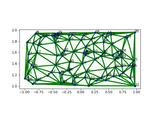
meshis a TriMesh object.Examples
A sample mesh is constructed by creating uniformly randomly distributed points on the rectangular domain [-1, 1] x [1, 2]. These points will constitute the vertices of the mesh, while its cells are the Delaunay triangles on the vertices.
>>> from grains.geometry import TriMesh
>>> msh = TriMesh(*TriMesh.sample_mesh(1))
The cells are drawn in greeen, in 3 points of line width, and the vertices of the mesh are shown in blue.
>>> msh.plot('go-', linewidth=3, markerfacecolor='b', vertex_labels=True)
>>> plt.show()
(Source code, png, hires.png, pdf)
Notes
The plotting is done by calling
triplot(), which internally makes a deep copy of the triangles. This increases the memory usage in case of many elements.
-
plot_field(component, *args, show_mesh=True, **kwargs)[source]¶ Plots a field on the mesh.
The aim of this method is to support basic post-processing for finite element visualization. Only the basic contour plot type is available. For vector or tensor fields, the components to be plotted must be chosen. For faster and more comprehensive plotting capabilities, turn to well-established scientific visualization software, such as ParaView or Mayavi. Another limitation of the
plot_field()method is that field values are assumed to be associated to the vertices of the mesh, which restricts us to \(P1\) Lagrange elements.- Parameters
component (int) – Positive integer, the selected component of the field to be plotted. Components are indexed from 0.
show_mesh (bool, optional) – If True, the underlying mesh is shown. The default is True.
ax (matplotlib.axes.Axes, optional) – The Axes instance the plot resides in. The default is None, in which case a new Axes within a new figure is created.
- Other Parameters
See them described in the :meth:`plot` method.
- Returns
None
See also
Examples
The following example considers the same type of mesh as in the example shown for
plot().>>> msh = TriMesh(*TriMesh.sample_mesh(1))
We pretend that the field is an analytical function, evaluated at the vertices.
>>> field = lambda x, y: 1 - (x + y**2) * np.sign(x)
>>> field = field(msh.vertices[:, 0], msh.vertices[:, 1])
We associate this field to the mesh and plot it with and without the mesh
>>> msh.associate_field(field, 'analytical field')
>>> _, (ax1, ax2) = plt.subplots(1, 2)
>>> msh.plot_field(0, 'bo-', ax=ax1, linewidth=1, markerfacecolor='k')
>>> msh.plot_field(0, ax=ax2, show_mesh=False)
>>> plt.show()
-
plot_options= {'ax': None, 'cell_labels': False, 'cell_legends': False, 'cell_sets': True, 'vertex_labels': False, 'vertex_legends': False, 'vertex_sets': True}
-
rotate(angle, point=(0, 0), inplace=False)[source]¶ Rotates a 2D mesh about a given point by a given angle.
- Parameters
angle (float) – Angle of rotation, in radians.
point (list or tuple, optional) – Coordinates of the point about which the mesh is rotated. If not given, it is the origin.
inplace (bool, optional) – If True, the vertex positions are updated in the mesh object. The default is False.
- Returns
rotated_vertices (ndarray) – Same format as the
verticesmember variable, with the requested rotation.
Notes
Rotating a point \(P\) given by its coordinates in the global coordinate system as \(P(x,y)\) around a point \(A(x,y)\) by an angle \(\alpha\) is done as follows.
1. The coordinates of \(P\) in the local coordinate system, the origin of which is \(A\), is expressed as
\[P(x',y') = P(x,y) - A(x,y).\]2. The rotation is performed in the local coordinate system as \(P'(x',y') = RP(x',y')\), where \(R\) is the rotation matrix:
\[\begin{split}R = \begin{pmatrix} \cos\alpha & -\sin\alpha \\ \sin\alpha & \hphantom{-}\cos\alpha \end{pmatrix}.\end{split}\]The rotated point \(P'\) is expressed in the original (global) coordinate system:
\[P'(x,y) = P'(x',y') + A(x,y).\]
-
static
sample_mesh(sample, param=100)[source]¶ Provides sample meshes.
- Parameters
sample (int) – Integer, giving the sample mesh to be considered. Possibilities:
param – Parameters to the sample meshes. Possibilities:
- Returns
nodes (ndarray) – 2D numpy array with 2 columns, each row corresponding to a vertex, and the two columns giving the Cartesian coordinates of the vertices.
cells (ndarray) – Cell-vertex connectivity in a 2D numpy array, in which each row corresponds to a cell and the columns are the vertices of the cells. It is assumed that all the cells have the same number of vertices.
-
scale(factor, inplace=False)[source]¶ Scales the geometry by modifying the coordinates of the vertices.
- Parameters
factor (float) – Each vertex coordinate is multiplied by this non-negative number.
inplace (bool, optional) – If True, the vertex positions are updated in the mesh object. The default is False.
- Returns
None.
-
grains.geometry._polygon_area(x, y)[source]¶ Computes the signed area of a non-self-intersecting, possibly concave, polygon.
Directly taken from http://rosettacode.org/wiki/Shoelace_formula_for_polygonal_area#Python
- Parameters
x, y (list) – Coordinates of the consecutive vertices of the polygon.
- Returns
float – Area of the polygon.
Warning
If numpy vectors are passed as inputs, the resulting area is incorrect! WHY?
Notes
The code is not optimized for speed and for numerical stability. Intended to be used to compute the area of finite element cells, in which case the numerical stability is not an issue (unless the cell is degenerate). As this function is called possibly as many times as the number of cells in the mesh, no input checking is performed.
Examples
>>> _polygon_area([0, 1, 1], [0, 0, 1])
0.5
-
grains.geometry.distance_matrix(points)[source]¶ A symmetric square matrix, containing the pairwise squared Euclidean distances among points.
- Parameters
points (ndarray) – 2D numpy array with 2 columns, each row corresponding to a point, and the two columns giving the Cartesian coordinates of the points.
- Returns
dm (ndarray) – Distance matrix.
See also
Examples
>>> points = np.array([[1, 1], [3, 0], [-1, -1]])
>>> distance_matrix(points)
array([[ 0.,  5.,  8.],
       [ 5.,  0., 17.],
       [ 8., 17.,  0.]])
-
grains.geometry.is_collinear(points, tol=None)[source]¶ Decides whether a set of points is collinear.
Works in any dimensions.
- Parameters
points (ndarray) – 2D numpy array with N columns, each row corresponding to a point, and the N columns giving the Cartesian coordinates of the point.
tol (float, optional) – Tolerance value passed to numpy’s matrix_rank function. This tolerance gives the threshold below which SVD values are considered zero.
- Returns
bool – True for collinear points.
See also
Notes
The algorithm for three points is from Tim Davis.
Examples
Two points are always collinear
>>> is_collinear(np.array([[1, 0], [1, 5]]))
True
Three points in 3D which are supposed to be collinear (returns false due to numerical error)
>>> is_collinear(np.array([[0, 0, 0], [1, 1, 1], [5, 5, 5]]), tol=0)
False
The previous example with looser tolerance
>>> is_collinear(np.array([[0, 0, 0], [1, 1, 1], [5, 5, 5]]), tol=1e-14)
True
-
grains.geometry.squared_distance(x, y)[source]¶ Squared Euclidean distance between two points.
For points \(x(x_1, ..., x_n)\) and \(y(y_1, ... y_n)\) the following metric is computed
\[\sum\limits_{i=1}^n (x_i - y_i)^2\]- Parameters
x, y (ndarray) – 1D numpy array, containing the coordinates of the two points.
- Returns
float – Squared Euclidean distance.
See also
Examples
>>> squared_distance(np.array([0, 0, 0]), np.array([1, 1, 1]))
3.0
Abaqus
Warning
This module will substantially be rewritten. See this issue.
This module allows to create and manipulate Abaqus input files through the Abaqus keywords, thereby providing automation. Note that it is not intended to be a complete API to Abaqus. If you want fine control over the whole Abaqus ecosystem, consult with the Abaqus Scripting Reference Guide (ASRG). However, ASRG needs Abaqus to be installed, moreover, you must use the Python interpreter embedded into Abaqus. That version of Python is very old even in the latest versions of Abaqus. Furthermore, if you need to use custom Python packages for your work, chances are high that they will not work with the embedded interpreter, and may even crash the installation. To use this module, no Abaqus installation is needed. In fact, only functions from the Python standard library are used.
The documentation of Abaqus version 2017 is hosted on the following website:
https://abaqus-docs.mit.edu/2017/English/SIMACAEEXCRefMap/simaexc-c-docproc.htm.
Throughout the documentation of this module (grains.abaqus), we will make references to
that website. If the links cease to exist, please let me know by
opening an issue.
Alternatively, once you have registered, you can browse the documentation on the
official website.
Classes
Geometrical operations on the mesh. |
|
Adds, removes, modifies materials. |
|
Handling analysis steps during the simulation. |
Functions
|
Obtains Abaqus keyword and its parameters. |
|
Input or output file validation. |
-
class
grains.abaqus.Geometry[source]¶ Bases:
objectGeometrical operations on the mesh.
-
_Geometry__format()¶ - Formats the material data in the Abaqus .inp format.
The internal representation of the material data in converted to a string understood by Abaqus.
- abaqus_formatlist
List of strings, each element of the list corresponding to a line (with
- line ending) in the Abaqus .inp file. In case of no
material, an empty list is returned.
The output is a list so that further concatenation operations are easy. If you want a string, merge the elements of the list:
output = ‘’.join(output)
This is what the show method does.
-
read(inp_file)[source]¶ Reads material data from an Abaqus .inp file.
- Parameters
inp_file (str) – Abaqus input (.inp) file to be created.
- Returns
None.
Notes
This method is designed to read material data. Although the logic could be used to process other properties (parts, assemblies, etc.) in an input file, they are not yet implemented in this class.
This method assumes that the input file is valid. If it is, the material data can be extacted. If not, the behavior is undefined: the program can crash or return garbage. This is by design: the single responsibility principle dictates that the validity of the input file must be provided by other methods. If the input file was generated from within Abaqus CAE, it is guaranteed to be valid. The write method of this class also ensures that the resulting input file is valid. This design choice also makes the program logic simpler. For valid syntax in the input file, check the Input Syntax Rules section in the Abaqus user’s guide.
To read material data from an input file, one has to identify the structure of .inp files in Abaqus. Abaqus is driven by keywords and corresponding data. For a list of accepted keywords, consult the Abaqus Keywords Reference Guide. There are three types of input lines in Abaqus:
keyword line: begins with a star, followed by the name of the keyword. Parameters, if any, are separated by commas and are given as parameter-value pairs. Keywords and parameters are not case sensitive. Example:
*ELASTIC, TYPE=ISOTROPIC, DEPENDENCIES=1
Some keywords can only be defined once another keyword has already been defined. E.g. the keyword ELASTIC must come after MATERIAL in a valid .inp file.
data line: immediately follows a keyword line. All data items must be separated by commas. Example:
-12.345, 0.01, 5.2E-2, -1.2345E1
- comment line: starts with ** and is ignored by Abaqus. Example:
** This is a comment line
Internally, the materials are stored in a dictionary. It holds the material data read from the file. The keys in this dictionary are the names of the materials, and the values are dictionaries themselves. Each such dictionary stores a behavior for the given material. E.g. an elastoplastic material is governed by an elastic and a plastic behavior. The parameters for each behavior are stored in a list.
-
scale(factor)[source]¶ Scales the geometry by modifying the coordinates of the nodes.
- Parameters
factor (float) – Each nodal coordinate is multiplied by this non-negative number.
- Returns
None.
Notes
The modification happens in-place.
-
write(output_file=None)[source]¶ Writes material data to an Abaqus .inp file.
- Parameters
output_file (str, optional) – Output file name to write the modifications into. If not given, the original file name is appended with ‘_mod’.
- Returns
None.
Notes
If the output file name is the same as the input file, the original .inp file will be overwritten. This is strongly not recommended.
The whole content of the original input file is read to memory. It might be a problem for very large .inp files. In that case, a possible implementation could be the following:
Remove old material data
Append new material data to the proper position in the file
Appending is automatically done at the end of the file. Moving the material description to the end of the file is not possible in general because defining materials cannot be done from any module, i.e. the *MATERIAL keyword cannot follow an arbitrary keyword. In this case, Abaqus throws an AbaqusException with the following message:
It can be suboption for the following keyword(s)/level(s): model
-
-
class
grains.abaqus.Material(from_Abaqus=False)[source]¶ Bases:
objectAdds, removes, modifies materials. Requirements: be able to - create an empty .inp file, containing only the materials - add materials to an existing .inp file
TODO: only document public attributes! .. attribute:: materials
materials, their behaviors and their parameters are stored here. Intended for internal representation. To view them, use the show method, to write them to an input file, use the write method.
- type
dict
Notes
The aim of this class is to programmatically add, remove, modify materials in a format understandable by Abaqus. This class does not target editing materials through a GUI (that can be done in Abaqus CAE).
-
_Material__format()¶ - Formats the material data in the Abaqus .inp format.
The internal representation of the material data in converted to a string understood by Abaqus.
- abaqus_formatlist
List of strings, each element of the list corresponding to a line (with
- line ending) in the Abaqus .inp file. In case of no
material, an empty list is returned.
The output is a list so that further concatenation operations are easy. If you want a string, merge the elements of the list:
output = ‘’.join(output)
This is what the show method does.
-
static
_Material__isnumeric(x)¶ Decides if the input is a scalar number.
- Parameters
x (any type) – Input to be tested.
- Returns
bool – True if the given object is a scalar number.
-
add_linearelastic(material, E, nu)[source]¶ Adds linear elastic behavior to a given material.
- Parameters
material (str) – Name of the material the behavior belongs to.
E (int, float) – Young’s modulus.
nu (int, float) – Poisson’s ratio.
- Returns
None.
-
add_material(material)[source]¶ Defines a new material by its name.
- Parameters
material (str) – Name of the material to be added. A material can have multiple behaviors (e.g. elastoplastic).
- Returns
None.
-
add_plastic(material, sigma_y, epsilon_p)[source]¶ Adds metal plasticity behavior to a given material.
- Parameters
material (str) – Name of the material the behavior belongs to.
sigma_y (int, float) – Yield stress.
epsilon_p (int, float) – Plastic strain.
- Returns
None.
-
static
add_sections(inp_file, output_file=None)[source]¶ Adds section definitions to an Abaqus .inp file.
Defines properties for elements by associating materials to them. The element set containing the elements for which the material behavior is being defined is assumed to have the same name as that of the material. E.g. if materials with names mat-1 and mat-2 exist, element sets with names mat-1 and mat-2 must also exist. If such element sets do not exist, Abaqus will throw a warning and the section assignment will not be successful.
- Parameters
inp_file (str) – Abaqus .inp file from which the materials should be removed.
output_file (str, optional) – Output file name to write the modifications into. If not given, the original file name is appended with ‘_mod’.
- Returns
None.
Notes
If fine control is required for associating custom material names to custom element set names, that can be done from the Abaqus GUI. The purpose of this method is automation for large number of element sets, each associated to a (possibly distinct) material. In that case, custom element set names are not reasonable any more, and having the same names for the element sets and for the materials is completely meaningful.
-
create(inp_file)[source] Creates empty Abaqus .inp file.
- Parameters
inp_file (str) – Abaqus input file to be created. If an extension is not given, the default .inp is used.
- Returns
None.
-
read(inp_file)[source] Reads material data from an Abaqus .inp file.
- Parameters
inp_file (str) – Abaqus input (.inp) file to be created.
- Returns
None.
Notes
This method is designed to read material data. Although the logic could be used to process other properties (parts, assemblies, etc.) in an input file, they are not yet implemented in this class.
This method assumes that the input file is valid. If it is, the material data can be extacted. If not, the behavior is undefined: the program can crash or return garbage. This is by design: the single responsibility principle dictates that the validity of the input file must be provided by other methods. If the input file was generated from within Abaqus CAE, it is guaranteed to be valid. The write method of this class also ensures that the resulting input file is valid. This design choice also makes the program logic simpler. For valid syntax in the input file, check the Input Syntax Rules section in the Abaqus user’s guide.
To read material data from an input file, one has to identify the structure of .inp files in Abaqus. Abaqus is driven by keywords and corresponding data. For a list of accepted keywords, consult the Abaqus Keywords Reference Guide. There are three types of input lines in Abaqus:
keyword line: begins with a star, followed by the name of the keyword. Parameters, if any, are separated by commas and are given as parameter-value pairs. Keywords and parameters are not case sensitive. Example:
*ELASTIC, TYPE=ISOTROPIC, DEPENDENCIES=1
Some keywords can only be defined once another keyword has already been defined. E.g. the keyword ELASTIC must come after MATERIAL in a valid .inp file.
data line: immediately follows a keyword line. All data items must be separated by commas. Example:
-12.345, 0.01, 5.2E-2, -1.2345E1
- comment line: starts with ** and is ignored by Abaqus. Example:
** This is a comment line
Internally, the materials are stored in a dictionary. It holds the material data read from the file. The keys in this dictionary are the names of the materials, and the values are dictionaries themselves. Each such dictionary stores a behavior for the given material. E.g. an elastoplastic material is governed by an elastic and a plastic behavior. The parameters for each behavior are stored in a list.
-
static
remove(inp_file, output_file=None)[source] Removes material definitions from an Abaqus .inp file.
- Parameters
inp_file (str) – Abaqus .inp file from which the materials should be removed.
output_file (str, optional) – Output file name to write the modifications into. If not given, the original file name is appended with ‘_mod’.
- Returns
None.
-
show()[source] Shows material data as it appears in the Abaqus .inp file.
- Returns
None.
-
write(output_file=None)[source] Writes material data to an Abaqus .inp file.
- Parameters
output_file (str, optional) – Output file name to write the modifications into. If not given, the original file name is appended with ‘_mod’.
- Returns
None.
Notes
If the output file name is the same as the input file, the original .inp file will be overwritten. This is strongly not recommended.
The whole content of the original input file is read to memory. It might be a problem for very large .inp files. In that case, a possible implementation could be the following:
Remove old material data
Append new material data to the proper position in the file
Appending is automatically done at the end of the file. Moving the material description to the end of the file is not possible in general because defining materials cannot be done from any module, i.e. the *MATERIAL keyword cannot follow an arbitrary keyword. In this case, Abaqus throws an AbaqusException with the following message:
It can be suboption for the following keyword(s)/level(s): model
-
class
grains.abaqus.Procedure(from_Abaqus=False)[source]¶ Bases:
objectHandling analysis steps during the simulation.
TODO: only document public attributes!
-
steps¶ analysis steps, each step collecting the necessary information. Intended for internal representation. To view them, use the
show()method, to write them to an input file, use thewrite()method.- Type
-
_Procedure__format()¶ - Formats the data in the Abaqus .inp format.
The internal representation of the steps data in converted to a string understood by Abaqus.
- abaqus_formatlist
List of strings, each element of the list corresponding to a line (with
- line ending)
in the Abaqus .inp file. In case of no data, an empty list is returned.
The output is a list so that further concatenation operations are easy. If you want a string, merge the elements of the list:
output = ''.join(output)This is what theshow()method does.
-
add_analysis(step, time_period=1.0, initial_increment=None, min_increment=0, max_increment=None)[source]¶ Adds an analysis type to a given step.
Note
Currently only static stress/displacement analysis is supported, indicated by the STATIC Abaqus keyword. No optional parameters are supported.
Todo
Check user inputs. Define exceptions (ValueError class) with the error messages Abaqus CAE throws.
- Parameters
step (str) – Name of the step the analysis type belongs to.
initial_increment (float, optional) – Initial time increment. This value will be modified as required if the automatic time stepping scheme is used. If this entry is zero or is not specified, a default value that is equal to the total time period of the step is assumed.
time_period (float, optional) – Time period of the step. The default is 1.0.
min_increment (float, optional) – Only used for automatic time incrementation. If ABAQUS/Standard finds it needs a smaller time increment than this value, the analysis is terminated. If this entry is zero, a default value of the smaller of the suggested initial time increment or 1e–5 times the total time period is assumed.
max_increment (float, optional) – Maximum time increment allowed. Only used for automatic time incrementation. If this value is not specified, no upper limit is imposed, i.e.
max_increment
= time_period
.
- Returns
None
Examples
>>> proc = Procedure()
>>> proc.create_step('Step-1', max_increments=1000)
>>> proc.add_analysis('Step-1', initial_increment=0.001, min_increment=1e-8)
-
add_boundary_condition(name, step, nodes, first_dof, last_dof=None, magnitude=0.0)[source]¶ Adds boundary condition to a given step.
Boundary conditions can be prescribed on node sets, using the Abaqus keyword BOUNDARY. Optional parameters are not supported.
Multiple boundary conditions can be given on the same node set. It is the responsibility of the user to ensure that the constraints are compatible.
Note
Currently, boundary conditions can only be defined in a user-defined step, and not in the initial step.
- Parameters
name (str) – Name of the boundary condition to be added. Boundary condition names must be unique.
step (str) – Name of the step the boundary condition belongs to.
nodes (str or int) – If a string, the label of the node set, if a positive integer, the label of a single node on which the boundary condition is prescribed.
first_dof (int) – First degree of freedom constrained.
last_dof (int, optional) – Last degree of freedom constrained. Not necessary to be given if only one degree of freedom is being constrained.
magnitude (float) – Magnitude of the variable. If this magnitude is a rotation, it must be given in radians. The default value is 1.0.
- Returns
None
Examples
Let us consider a two-dimensional structure, fixed on a part of its boundary (called ‘left’), and displaced on another part (called ‘right’). First, we create an analysis step (named ‘Step-1’).
>>> proc = Procedure()
>>> proc.create_step('Step-1', max_increments=1000)
Now, we prescribe the zero displacements.
>>> proc.add_boundary_condition('fixed', 'Step-1', 'left', first_dof=1, last_dof=2)
Since we did not specify the magnitude of the displacement components, they are zero by default. The other boundary condition prescribes different values for the horizontal and vertical components. Hence, they are given separately.
>>> proc.add_boundary_condition('pulled_right', 'Step-1', 'right', first_dof=1, magnitude=2)
>>> proc.add_boundary_condition('fixed_right', 'Step-1', 'right', first_dof=2, magnitude=0)
Note that we can also prescribe boundary conditions at a particular node, e.g.
>>> proc.add_boundary_condition('at_node', 'Step-1', 1, first_dof=2, magnitude=-1.2)
where we set the vertical displacement component to -1.2 at node 1.
-
create_step(name, nlgeom=False, max_increments=100)[source]¶ Defines a new step.
A step is the fundamental part of the simulation workflow in Abaqus. Among the available options, only the NLGEOM and INC options are supported currently.
Todo
Check in the
write()method whether every step contains an analysis, as this is required by Abaqus.- Parameters
name (str) – Name of the analysis step to be added. Step names must be unique.
nlgeom (bool, optional) – Omit this parameter or set to False to perform a geometrically linear analysis during the current step. Set it to True to indicate that geometric nonlinearity should be accounted for during the step. Once the
nlgeomoption has been switched on, it will be active during all subsequent steps in the analysis. The default is False.max_increments (int) – The analysis will stop if the maximum number of increments is exceeded before the complete solution for the step has been obtained. The default is 100.
- Returns
None
-
read(inp_file)[source]¶ Reads procedure data from an Abaqus .inp file.
- Parameters
inp_file (str) – Abaqus input (.inp) file to be created.
- Returns
None.
Notes
This method is designed to read material data. Although the logic could be used to process other properties (parts, assemblies, etc.) in an input file, they are not yet implemented in this class.
This method assumes that the input file is valid. If it is, the material data can be extacted. If not, the behavior is undefined: the program can crash or return garbage. This is by design: the single responsibility principle dictates that the validity of the input file must be provided by other methods. If the input file was generated from within Abaqus CAE, it is guaranteed to be valid. The write method of this class also ensures that the resulting input file is valid. This design choice also makes the program logic simpler. For valid syntax in the input file, check the Input Syntax Rules section in the Abaqus user’s guide.
To read material data from an input file, one has to identify the structure of .inp files in Abaqus. Abaqus is driven by keywords and corresponding data. For a list of accepted keywords, consult the Abaqus Keywords Reference Guide. There are three types of input lines in Abaqus:
keyword line: begins with a star, followed by the name of the keyword. Parameters, if any, are separated by commas and are given as parameter-value pairs. Keywords and parameters are not case sensitive. Example:
*ELASTIC, TYPE=ISOTROPIC, DEPENDENCIES=1
Some keywords can only be defined once another keyword has already been defined. E.g. the keyword ELASTIC must come after MATERIAL in a valid .inp file.
data line: immediately follows a keyword line. All data items must be separated by commas. Example:
-12.345, 0.01, 5.2E-2, -1.2345E1
- comment line: starts with ** and is ignored by Abaqus. Example:
** This is a comment line
Internally, the materials are stored in a dictionary. It holds the material data read from the file. The keys in this dictionary are the names of the materials, and the values are dictionaries themselves. Each such dictionary stores a behavior for the given material. E.g. an elastoplastic material is governed by an elastic and a plastic behavior. The parameters for each behavior are stored in a list.
-
show()[source]¶ Shows the text for the step module, as it appears in the Abaqus .inp file.
- Returns
None.
-
write(output_file=None)[source]¶ Writes step definition data to an Abaqus .inp file.
- Parameters
output_file (str, optional) – Output file name to write the modifications into. If not given, the original file name is appended with ‘_mod’.
- Returns
None.
Notes
If the output file name is the same as the input file, the original .inp file will be overwritten. This is strongly not recommended.
The whole content of the original input file is read to memory. It might be a problem for very large .inp files. In that case, a possible implementation could be the following:
Remove old material data
Append new material data to the proper position in the file
Appending is automatically done at the end of the file. Moving the material description to the end of the file is not possible in general because defining materials cannot be done from any module, i.e. the *MATERIAL keyword cannot follow an arbitrary keyword. In this case, Abaqus throws an AbaqusException with the following message:
It can be suboption for the following keyword(s)/level(s): model
-
DIC
This module is used to process field values obtained by digital image correlation (DIC). Plotting, comparison with numerical solutions, etc. are implemented.
Functions
|
Plots a scalar strain field. |
-
class
grains.dic.DIC(u, v)[source]¶ Bases:
objectPerforms operations on digital image correlation data.
- Parameters
u, v (ndarray) – The two components of the displacement field, discretized on a rectangular grid.
- Raises
ValueError – If the displacement components are not discretized on the same grid or if the grid size is not at least 3-by-3. This latter requirement is not a problem in practice (which camera is not capable of shooting photos in 9 pixels resolution?), while it allows the evaluation of the numerical derivatives with second order accuracy on the boundaries too.
Notes
Throughout the class methods, the following terms are used. When not precised, image refers to the DIC data plotted as an image. We can perceive the image as a pixel grid, in which the vertices are the centres of the pixels. An image coordinate system \((X,Y)\) can be defined on this grid such that the vertices have integer coordinates, the origin \(A\) is at the top left hand corner, and the \(Y\)-axis points towards the right, while the \(X\)-axis points to the bottom. When the experimental result is compared with a numerical solution (assumed to be available at the nodes of a mesh), one needs to map values defined on the DIC grid onto the nodes of the mesh, and vice versa. The mesh exists on the physical domain, for which a physical coordinate system \((x,y)\) is attached to. Hence, there is a need to express \((X,Y)\) in terms of \((x,y)\). Let \(A(a_x,a_y)\) be the origin of the \((X,Y)\) coordinate system given in terms of the \(x,y\) coordinates, and \(s[\mathrm{pixel/mm}]\) is the scale for the DIC image. The coordinate transformation is then given by
\[\begin{split}\begin{gather} x = a_x + \frac{Y}{s} \\ y = a_y - \frac{X}{s} \end{gather}\end{split}\]The DIC grid in the physical coordinate system \((x,y)\) is called physical grid.
It should be noted that the special alignment of \((x,y)\) with respect to \((X,Y)\) is not a major constraint. In practical applications (when a Cartesian coordinate system is used), the orientation of \((x,y)\) in this way is a convention.
-
static
equivalent_strain(strain_tensor, strain_measure)[source]¶ Computes a scalar quantity from the strain tensor.
- Parameters
strain_tensor (ndarray) – Components of the strain tensor \(\boldsymbol{\varepsilon}\) as an \(m \times n \times 3\) array. The first two dimensions correspond to the grid points they are determined at, the third dimension gives the components of the tensor in the following order: \(\varepsilon_{11}, \varepsilon_{12}, \varepsilon_{22}\).
strain_measure ({‘von Mises’}) – One of the following strain measures.
‘von Mises’
\[\varepsilon_M := \sqrt{\frac{2}{3} \boldsymbol{\varepsilon}^{\mathrm{dev}} : \boldsymbol{\varepsilon}^{\mathrm{dev}}} = \sqrt{\frac{2}{3} \left( \boldsymbol{\varepsilon}:\boldsymbol{\varepsilon} - \frac{1}{3}(\mathrm{tr} \boldsymbol{\varepsilon})^2 \right)}\]where \(\boldsymbol{\varepsilon}^{\mathrm{dev}}\) is the deviatoric part of the strain tensor. This can further be simplified (see the notes below) to
\[\varepsilon_M = \frac{2}{3}\sqrt{\varepsilon_{11}^2 + \varepsilon_{22}^2 + 3\varepsilon_{12}^2 - \varepsilon_{11}\varepsilon_{22}}\]
- Returns
ndarray – Equivalent strain at the grid points, given as an \(m \times n\) numpy array.
See also
Notes
Under plane stress conditions, \(\varepsilon_{33}\) is not zero, but it is computed as
\[\varepsilon_{33} = -\frac{\nu}{E}(\sigma_{11} + \sigma_{22})\]Since the stresses are not known from the DIC, one must settle with plane strain conditions where \(\varepsilon_{33} = 0\). This is what we follow in the
DICclass. We remark that in stereo-DIC multiple cameras are used, which allows the measurement of \(\varepsilon_{33}\).
-
plot_displacement(component, ax=None)[source]¶ Plots a component of the displacement field.
- Parameters
component ({1, 2}) – Component to be plotted, where 1 corresponds to the first, 2 corresponds to the second component of the displacement field.
ax (matplotlib.axes.Axes, optional) – The Axes instance the grid resides in. The default is None, in which case a new Axes within a new figure is created.
- Returns
None
See also
-
plot_physicalgrid(ax=None)[source]¶ Plots the DIC grid in the physical coordinate system.
This method is only available once the relation between the image coordinate system and the physical coordinate system has been set up by the
set_transformation()method.- Parameters
ax (matplotlib.axes.Axes, optional) – The Axes instance the grid resides in. The default is None, in which case a new Axes within a new figure is created.
- Returns
ax (matplotlib.axes.Axes)
See also
Notes
See in the
plot_pixelgrid()method.
-
plot_pixelgrid(ax=None)[source]¶ Plots the DIC grid in the image coordinate system.
- Parameters
ax (matplotlib.axes.Axes, optional) – The Axes instance the grid resides in. The default is None, in which case a new Axes within a new figure is created.
- Returns
ax (matplotlib.axes.Axes)
See also
Notes
For a DIC image with \(m \times n\) number of pixels, the number of grid lines is \((m + 1) + (n + 1)\). Plotting all these lines would not only slow down the program, it would also make the grid practically indistinguishable from a filled rectangle. Therefore, for high resolution images, only grid lines around the boundary of the image are plotted. The target resolution above which this strategy is used can be given in the class constructor.
-
plot_strain(component, minval=None, maxval=None, colorbar=True)[source]¶ Plots a component of the infinitesimal strain tensor.
The partial derivatives of the displacement field are computed with numerical differentiation.
- Parameters
component (tuple, {(1,1), (1,2), (2,1), (2,2)}) – Component to be plotted, where
(1,1) denotes \(\varepsilon_{11}\)
(1,2) and (2,1) denote \(\varepsilon_{12} = \varepsilon_{21}\)
(2,2) denotes \(\varepsilon_{22}\)
for the infinitesimal strain tensor
\[\begin{split}\varepsilon = \begin{pmatrix} \varepsilon_{11} & \varepsilon_{12} \\ \varepsilon_{21} & \varepsilon_{22} \end{pmatrix}\end{split}\]minval, maxval (float, optional) – Set the color scaling for the image by fixing the values that map to the colormap color limits. If
minvalis not provided, the limit is determined from the minimum value of the data. Similarly formaxval.colorbar (bool, optional) – If True, a horizontal colorbar is placed below the strain map. The default is True.
- Returns
None
See also
Deprecated since version 1.1.0: This will be removed in 1.3.0. This method will be modified to perform the plotting only. The computation of the various strain measures will be done in the
strain()method. The function that replaces this function will keep the same name and is currently implemented outside this class.
-
plot_superimposedmesh(mesh, *args, **kwargs)[source]¶ Plots the DIC grid with a mesh superimposed on it.
Since the finite element mesh represents a physical domain, the DIC grid is plotted in the physical coordinate system, which is determined by the
set_transformation()method.Note
Maybe no need to couple this module with the geometry module just for the sake of this function. It is probably easier to simply pass the nodes and the elements, and call triplot.
- Parameters
mesh (Mesh) – A subclass of
grains.geometry.Meshto be plotted along with the physical DIC grid.args (optional) – The same as for
matplotlib.axes.Axes.plot(). The settings given here influence the mesh plotting.kwargs (optional) – The same as for
matplotlib.axes.Axes.plot(). The settings given here influence the mesh plotting.
- Returns
ax (matplotlib.axes.Axes) – The Axes object on which the plot is drawn.
See also
Examples
Let us create a grid and a random mesh (the same as in the Examples section of the
project_onto_mesh()).>>> from grains.dic import DIC >>> from grains.geometry import TriMesh >>> x_grid, y_grid = np.mgrid[-1:1:100j, 1:2:50j] >>> exact_solution = lambda x, y: 1 - (x + y**2) * np.sign(x) >>> grid = DIC(np.random.rand(*np.shape(x_grid.T)), np.random.rand(*np.shape(x_grid.T))) >>> grid.set_transformation((-1, 2), 50) >>> n_nodes = 100 # modify this to see how good the interpolated solution is >>> msh = TriMesh(*TriMesh.sample_mesh(1, n_nodes)) >>> grid.plot_superimposedmesh(msh, linewidth=3, markerfacecolor='b') >>> plt.show()
(Source code, png, hires.png, pdf)
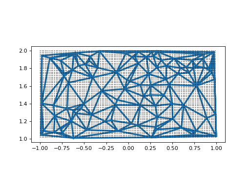
-
project_onto_grid(nodes, nodal_values, method='linear')[source]¶ Project a numerically computed field onto the DIC grid.
Todo
Use the example code of this method to create the plotting method of this class. When done, rewrite the example with the methods.
- Parameters
nodes (ndarray) – 2D numpy array with 2 columns, each row corresponding to a node of the mesh, and the two columns giving the Cartesian coordinates of the nodes.
nodal_values (ndarray) – 1D numpy array (vector), the numerically computed field at the nodes of the mesh.
method ({‘nearest’, ‘linear’, ‘cubic’}, optional) – Type of the interpolation. The default is linear.
- Returns
ndarray – 2D numpy array, the projected field values at the physical DIC grid points.
Examples
The DIC grid and the nodal finite element values (interpolated in-between, which is an errenous way to visualize discontinuous functions) can be seen in the upper left and lower left figures, respectively.
>>> from grains.dic import DIC
>>> from grains.geometry import TriMesh
>>> x_grid, y_grid = np.mgrid[-1:1:100j, 1:2:50j]
>>> exact_solution = lambda x, y: 1 - (x + y**2) * np.sign(x)
>>> grid = DIC(exact_solution(x_grid, y_grid).T, exact_solution(x_grid,y_grid).T)
>>> grid.set_transformation((-1, 2), 50)
The finite element solution is obtained at the nodes (upper right figure) of the mesh. Here, we assumed that the nodes are sampled from a uniformly random distribution on \([-1,1] \times [1, 2]\).
>>> n_nodes = 100 # modify this to see how good the interpolated solution is
For the sake of this example, we also assume that the nodal values are “exact”, i.e. they admit the function values at the nodes. In reality, of course, this will not be the case, but this allows us to investigate the effect moving from the FE mesh to the DIC grid.
>>> mesh = TriMesh(*TriMesh.sample_mesh(1, n_nodes))
>>> fe_values = exact_solution(mesh.vertices[:, 0], mesh.vertices[:, 1])
>>> mesh.associate_field(fe_values)
>>> interpolated = grid.project_onto_grid(mesh.vertices, fe_values, method='linear')
The FE field available at the nodes are interpolated at the DIC grid points, as shown in the lower right figure. Note that no extrapolation is performed, so values are not computed at the grid points lying outside the convex hull of the finite element nodes.
>>> ax = []
>>> ax.append(plt.subplot(221))
>>> plt.plot(x_grid, y_grid, 'k.', ms=1)
>>> plt.title('DIC grid')
>>> ax.append(plt.subplot(222))
>>> plt.plot(mesh.vertices[:, 0], mesh.vertices[:, 1], 'k.', ms=1)
>>> plt.title('FE nodes')
>>> ax.append(plt.subplot(223))
>>> mesh.plot_field(0, ax=ax[-1])
>>> plt.title('FE field')
>>> ax.append(plt.subplot(224))
>>> plt.imshow(interpolated, extent=(-1, 1, 1, 2), origin='lower', vmin=-4, vmax = 5)
>>> plt.title('FE field interpolated at the DIC grid')
>>> plt.tight_layout()
>>> for a in ax:
...     a.set_aspect('equal', 'box')
>>> plt.show()
(Source code, png, hires.png, pdf)
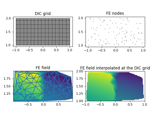
You are invited to modify this example to simulate a finer mesh by increasing
n_nodes. Also try different interpolation techniques.
-
project_onto_mesh(nodes, method='linear')[source]¶ Project the experimental displacement field onto a mesh.
- Parameters
nodes (ndarray) – 2D numpy array with 2 columns, each row corresponding to a node of the mesh, and the two columns giving the Cartesian coordinates of the nodes.
- Returns
u_nodes, v_nodes (ndarray) – 1D numpy arrays (vectors), the components of the projected displacement field at the given
nodes.method ({‘nearest’, ‘linear’, ‘cubic’}, optional) – Type of the interpolation. The default is linear.
See also
Examples
Suppose we have measured field data, obtained by DIC. The experimental field values are obtained as an image. The pixel centers of this image form a grid, each grid point having an associated scalar value, the value of the measured field. In this example, we pretend that the measured field is given as a function. The DIC grid and the measured field values can be seen in the upper left and lower left figures, respectively.
>>> from grains.dic import DIC
>>> from grains.geometry import TriMesh
>>> x_grid, y_grid = np.mgrid[-1:1:100j, 1:2:50j]
>>> exact_solution = lambda x, y: 1 - (x + y**2) * np.sign(x)
>>> grid = DIC(exact_solution(x_grid, y_grid).T, exact_solution(x_grid,y_grid).T)
The finite element solution is obtained at the nodes (upper right figure) of the mesh. Here, we assumed that the nodes are sampled from a uniformly random distribution on \([-1,1] \times [1, 2]\).
>>> n_nodes = 100  # modify this to see how good the interpolated solution is
>>> mesh = TriMesh(*TriMesh.sample_mesh(1, n_nodes))
For the sake of this example, we also assume that the nodal values are “exact”, i.e. they are the function values at the nodes. In reality, of course, this will not be the case, but this allows us to investigate the effect moving from the FE mesh to the DIC grid.
>>> grid.set_transformation((-1, 2), 50)
>>> fe_values = exact_solution(mesh.vertices[:, 0], mesh.vertices[:, 1])
>>> interpolated = grid.project_onto_mesh(mesh.vertices, 'nearest')
The FE solution available at the nodes are interpolated at the DIC grid points, as shown in the lower right figure. Interpolation with continuous functions cannot resolve well the discontinuity present in the “exact solution”, i.e. in the measurement data. A discontinuous manufactured solution was intentionally prepared to illustrate this.
>>> ax = []
>>> ax.append(plt.subplot(221))
>>> grid.plot_physicalgrid(ax[0])
>>> plt.title('DIC grid')
>>> ax.append(plt.subplot(222))
>>> mesh.plot('k.', ax=ax[1], markersize=1)
>>> plt.title('FE nodes')
>>> ax.append(plt.subplot(223))
>>> plt.imshow(exact_solution(x_grid, y_grid).T, extent=(-1, 1, 1, 2), origin='lower',
...            vmin=-4, vmax = 5)
>>> plt.title('Exact solution on the DIC grid')
>>> ax.append(plt.subplot(224))
>>> interpolated[0][np.isnan(interpolated[0])] = 0
>>> mesh.associate_field(interpolated[0])
>>> mesh.plot_field(0, show_mesh=False, ax=ax[3])
>>> plt.title('FE solution interpolated at the DIC grid')
>>> plt.show()
(Source code, png, hires.png, pdf)

You are invited to modify this example to simulate a finer mesh by increasing
n_nodes. Also try different interpolation techniques.
-
set_transformation(origin, pixels_per_physicalunit)[source]¶ Sets the transformation rule between the pixel and the physical coordinate systems.
To determine the position and the size of the DIC image in the physical space, a transformation rule needs to be given, as described in the Notes section of the
DICclass.- Parameters
origin (tuple) – 2-tuple of float, the coordinates of the origin of the DIC grid (upper left corner) in the physical coordinate system.
pixels_per_physicalunit (float)
- Returns
None
-
strain(strain_measure)[source]¶ Computes the strain tensor from the displacement vector.
The symmetric strain tensor \(\boldsymbol{\varepsilon}\) with components
\[\begin{split}\boldsymbol{\varepsilon} = \begin{pmatrix} \varepsilon_{11} & \varepsilon_{12} \\ \varepsilon_{21} & \varepsilon_{22} \end{pmatrix}\end{split}\]is computed for the given strain measure. The partial derivatives of the displacement field \((u,v)\), available on an \(m \times n\) grid, are computed with numerical differentiation with second order accuracy.
- Parameters
strain_measure ({‘infinitesimal’, ‘Green-Lagrange’}) – One of the following strain measures.
‘infinitesimal’
\[\begin{split}\varepsilon_{11} = \frac{\partial u}{\partial x} \\ \varepsilon_{12} = \frac{1}{2} \left( \frac{\partial u}{\partial y} + \frac{\partial v}{\partial x} \right) \\ \varepsilon_{22} = \frac{\partial v}{\partial y} \\\end{split}\]‘Green-Lagrange’
\[\begin{split}\varepsilon_{11} = \frac{1}{2} \left( 2\frac{\partial u}{\partial x} + \left(\frac{\partial u}{\partial x}\right)^2 + \left(\frac{\partial v}{ \partial x}\right)^2 \right) \\ \varepsilon_{12} = \frac{1}{2} \left( \frac{\partial u}{\partial y} + \frac{\partial v}{\partial x} + \frac{\partial u}{\partial x} \frac{\partial u}{\partial y} + \frac{\partial v}{\partial x} \frac{\partial v}{\partial y} \right) \\ \varepsilon_{22} = \frac{1}{2} \left( 2\frac{\partial v}{\partial y} + \left(\frac{\partial u}{\partial y}\right)^2 + \left(\frac{\partial v}{ \partial y}\right)^2 \right) \\\end{split}\]
- Returns
strain_tensor (ndarray) – Components of the strain tensor as an \(m \times n \times 3\) array. The first two dimensions correspond to the grid points they are determined at, the third dimension gives the components of the tensor in the following order: \(\varepsilon_{11}, \varepsilon_{12}, \varepsilon_{22}\).
See also
Notes
The derivatives of the displacement field are computed in the the physical coordinate system.
Examples
Consider a rectangular body with a linear displacement function in horizontal direction and no displacement vertically. The deformation of the body is such that only the horizontal strain is nonzero.
>>> u = np.array([[0, 1e-3, 2e-3, 3e-3], [0, 1e-3, 2e-3, 3e-3], [0, 1e-3, 2e-3, 3e-3]])
>>> v = np.zeros((3,4))
>>> d = DIC(u, v)
>>> E = d.strain('infinitesimal')
>>> E[:, :, 0]
array([[0.001, 0.001, 0.001, 0.001],
       [0.001, 0.001, 0.001, 0.001],
       [0.001, 0.001, 0.001, 0.001]])
>>> np.allclose(E[:, :, 2], 0)
True
>>> np.allclose(E[:, :, 1], 0)
True
The Green-Lagrange strain tensor is slightly different. Comparing with the infinitesimal strain tensor shows how good the assumption of small deformations is.
>>> E_gl = d.strain('Green-Lagrange')
>>> E_gl[:, :, 0] - E[:, :, 0]
array([[5.e-07, 5.e-07, 5.e-07, 5.e-07],
       [5.e-07, 5.e-07, 5.e-07, 5.e-07],
       [5.e-07, 5.e-07, 5.e-07, 5.e-07]])
The other two strain components remain zero.
>>> np.allclose(E_gl[:, :, 1:2], 0)
True
-
grains.dic.plot_strain(strain, minval=None, maxval=None, colorbar=True, label='')[source]¶ Plots a scalar strain field.
- Parameters
strain (ndarray) – Scalar strain field sampled on an m-by-n grid, given as a 2D numpy array.
minval, maxval (float, optional) – Set the color scaling for the image by fixing the values that map to the colormap color limits. If
minvalis not provided, the limit is determined from the minimum value of the data. Similarly formaxval.colorbar (bool, optional) – If True, a horizontal colorbar is placed below the strain map. The default is True.
label (str, optional) – Label describing the strain field. LaTeX code is also accepted, e.g. r’$varepsilon_{yy}$’. If not given, no text is displayed.
- Returns
None
See also
Deprecated since version 1.1.0: This will be removed in 1.3.0. This function will be a static method of the
DICclass. See also the deprecation warning ofDIC.plot_strain().
Simulation
Functions
Yield stresses and average grain diameters from Pierre’s thesis. |
|
Determines the two Hall-Petch constants. |
|
Computes the yield stress from the Hall-Petch relation. |
|
Plots the Hall-Petch formula for given grain sizes and yield stresses. |
|
Extends or crops the domain an image fills. |
|
Characterizes the intergranular/intragranular deformations. |
-
grains.simulation.change_domain(image, left, right, bottom, top, padding_value=nan)[source]¶ Extends or crops the domain an image fills.
The original image is extended, cropped or left unchanged in the left, right, bottom and top directions by padding the corresponding 2D or 3D array with a given value or removing existing elements. Non-integer image length is avoided by rounding up. This choice prevents ending up with an empty image during cropping or no added pixel during extension.
- Parameters
image (ndarray) – 2D or 3D numpy array representing the original image.
left, right (float) – When positive, the domain is extended, when negative, the domain is cropped by the given value relative to the image width.
bottom, top (float) – When positive, the domain is extended, when negative, the domain is cropped by the given value relative to the image height.
padding_value (float, optional) – Value for the added pixels. The default is numpy.nan.
- Returns
changed_image (ndarray) – 2D or 3D numpy array representing the modified domain.
Examples
Crop an image at the top, extended it at the bottom and on the left, and leave it unchanged on the right. Note the rounding for non-integer pixels.
>>> import numpy as np
>>> image = np.array([[0.1, 0.2, 0.3], [0.4, 0.5, 0.6], [0.7, 0.8, 0.9]])
>>> modified = change_domain(image, 0.5, 0, 1/3, -1/3, 0)
>>> image  # no in-place modification, the original image is not overwritten
array([[0.1, 0.2, 0.3],
       [0.4, 0.5, 0.6],
       [0.7, 0.8, 0.9]])
>>> modified
array([[0. , 0. , 0.4, 0.5, 0.6],
       [0. , 0. , 0.7, 0.8, 0.9],
       [0. , 0. , 0. , 0. , 0. ]])
-
grains.simulation.data_Pierre()[source]¶ Yield stresses and average grain diameters from Pierre’s thesis.
- Returns
sigma_y (list of floats) – Yield stresses.
d (list of floats) – Diameters of the grains.
-
grains.simulation.hallpetch(sigma_0, k, d)[source]¶ Computes the yield stress from the Hall-Petch relation.
- Parameters
sigma_0 (float) – Starting stress for dislocation movement (material constant).
k (float) – Strengthening coefficient (material constant).
d (float or list of floats) – Diameter of the grain.
- Returns
sigma_y (float or list of floats) – Yield stress.
-
grains.simulation.hallpetch_constants(sigma_y, d)[source]¶ Determines the two Hall-Petch constants. Given available measurements for the grains sizes and the yield stresses, the two constants in the Hall-Petch formula are computed.
- Parameters
sigma_y (list of floats) – Yield stresses.
d (list of floats) – Diameters of the grains.
- Returns
sigma_0 (float) – Starting stress for dislocation movement (material constant).
k (float) – Strengthening coefficient (material constant).
Notes
If two data points are given in the inputs (corresponding to two measurements), the output parameters have unique values:
k = (sigma_y[0] - sigma_y[1]) / (1/sqrt(d[0]) - 1/sqrt(d[1])) sigma_0 = sigma_y[0] - k/sqrt(d[0])
If there are more than two measurements, the resulting linear system is overdetermined. In both cases, the outputs are determined using least squares fitting.
-
grains.simulation.hallpetch_plot(sigma_y, d, units=('MPa', 'mm'))[source]¶ Plots the Hall-Petch formula for given grain sizes and yield stresses.
- Parameters
sigma_y (ndarray) – Yield stresses.
d (ndarray) – Grain diameters.
units (2-tuple of str, optional) – Units for the yield stress and the grain diameters. The default is (“MPa”,”mm”).
- Returns
fig (matplotlib.figure.Figure) – The figure object is returned in case further manipulations are necessary.
-
grains.simulation.nature_of_deformation(microstructure, strain_field, interface_width=3, visualize=True)[source]¶ Characterizes the intergranular/intragranular deformations.
To decide whether the strain localization is intergranular (happens along grain boundaries, also called interfaces) or intragranular in a given microstructure, the strain field is projected on the microstructure. Here, by strain field we mean a scalar field, often called equivalent strain that is derived from a strain tensor.
It is irrelevant for this function whether the strain field is obtained from a numerical simulation or from a (post-processed) full-field measurement. All what matters is that the strain field be available on a grid of the same size as the microstructure.
The strain field is assumed to be localized on an interface if its neighborhood, with band width defined by the user, contains higher strain values than what is outside the band (i.e. the grain interiors). A too large band width identifies small grains to have boundary only, without any interior. This means that even if the strain field in reality localizes inside such small grains, the localization is classified as intergranular. However, even for extreme deformations, one should not expect that the strain localizes on an interface with a single-point width. Moreover, using a too small band width is susceptible to the exact position of the interfaces, which are extracted from the grain microstructure. A judicial balance needs to be achieved in practice.
- Parameters
microstructure (ndarray) – Labelled image corresponding to the segmented grains in a grain microstructure.
strain_field (ndarray) – Discrete scalar field of the same size as the
microstructure.interface_width (int, optional) – Thickness of the band around the interfaces.
visualize (bool, optional) – If True, three plots are created. Two of them show the deformation field within the bands and outside the bands. They are linked together, so when you pan or zoom on one, the other plot will follow. The third plot contains two histograms on top of each other, giving the frequency of the strain values within the bands and outside the bands.
- Returns
boundary_strain (ndarray) – Copy of
strain_field, but values outside the band are set to NaN.bulk_strain (ndarray) – Copy of
strain_field, but values within the band are set to NaN.bands (ndarray) – Boolean array of the same size as
strain_field, with True values corresponding to the band.
See also
grains.dic.DIC.strain()Computes a strain tensor from the displacement field.
grains.dic.DIC.equivalent_strain()Extracts a scalar quantity from a strain tensor.
matplotlib.pyplot.hist()Plots a histogram.
Notes
From the modelling viewpoint, it is important to know whether the strain localizes to the grain boundaries or it is dominant within the grains as well. In the former case, simplifications in the models save computational time in the simulations.
In dynamics, the evolution of the strain field is relevant. E.g. an initially intergranular deformation can turn into diffuse localization that occurs within the grains as well. In that case, a strain field must be obtained at each time step, and this function can be called for each such instance.
Examples
The following figure was created by this function with
visualizeset to True andband_widthchosen to be 3.

Utilities
This module provides general utility functions used by the grains package. The specific helper functions reside in the proper module. For example, a function that works on a general list goes here, but a computational geometry algorithm goes to the geometry module. The functions in the utils module can be interesting for other projects too, partly because of their general scope, and partly because of the few dependencies.
Functions
Set of duplicate elements in a sequence. |
|
Return True for False values and False for True values in a list. |
|
Index a list by another list. |
|
Merge a list of lists to a single list. |
|
Return the indices that would sort a list or a tuple. |
|
Apply a function to each member of an iterable in-place. |
|
Finds indices of non-unique elements in a 1D or 2D ndarray. |
|
Compares keyword arguments with defaults. |
|
Creates a zip archive from a single file. |
|
Decompresses the contents of a zip archive into the current directory. |
|
Decompresses the contents of a zip archive into a dictionary. |
|
Neighboring points to a grid point. |
-
grains.utils.argsorted(sequence, reverse=False)[source]¶ Return the indices that would sort a list or a tuple.
Implementation is taken from https://stackoverflow.com/a/6979121/4892892.
- Parameters
sequence (list, tuple) – Input sequence in which the sorted indices to be found.
reverse (bool) – If set to True, then the elements are sorted as if each comparison was reversed.
- Returns
list – List of indices that would sort the input list/tuple.
See also
Examples
>>> argsorted([2, 1.1, 1.1])
[1, 2, 0]
>>> argsorted([2, 1.1, 1.1], reverse=True)
[0, 1, 2]
>>> argsorted(())
[]
-
grains.utils.compress(filename, level=9)[source]¶ Creates a zip archive from a single file.
- Parameters
filename (str) – Name of the file to be compressed.
level (int, optional) – Level of compression. Integers 0 through 9 are accepted. The default is 9.
- Returns
None.
See also
-
grains.utils.decompress(filename, path=None)[source]¶ Decompresses the contents of a zip archive into the current directory.
- Parameters
filename (str) – Name of the zip archive.
path (str, optional) – Directory to extract to. The default is the directory the function is called from.
See also
-
grains.utils.decompress_inmemory(filename)[source]¶ Decompresses the contents of a zip archive into a dictionary.
- Parameters
filename (str) – Name of the zip archive.
- Returns
data (dict) – The keys of the dictionary are the compressed file names (without extension), the corresponding values are their contents.
See also
-
grains.utils.duplicates(sequence)[source]¶ Set of duplicate elements in a sequence.
- Parameters
sequence (sequence types (list, tuple, string, etc.)) – Sequence possibly containing repeating elements.
- Returns
set – Set of unique values.
Notes
Copied from https://stackoverflow.com/a/9836685/4892892
Examples
Note that the order of the elements in the resulting set does not matter.
>>> a = [1, 2, 3, 2, 1, 5, 6, 5, 5, 5]  # list
>>> duplicates(a)
{1, 2, 5}
>>> a = (1, 1, 0, -1, -1, 0)  # tuple
>>> duplicates(a)
{0, 1, -1}
>>> a = 'abbcdkc'  # string
>>> duplicates(a)
{'c', 'b'}
-
grains.utils.flatten_list(nested_list)[source]¶ Merge a list of lists to a single list.
- Parameters
nested_list (list) – List containing other lists.
- Returns
list – Flattened list.
Notes
Only a single level (i.e. list of lists) is handled, see the second example.
Several methods, such as list comprehension, monoid and loops, are proposed in https://stackoverflow.com/questions/952914/how-to-make-a-flat-list-out-of-list-of-lists. Here, the list comprehension approach is used.
Examples
>>> nested_list = [['some'], ['items']]
>>> flatten_list(nested_list)
['some', 'items']
>>> multiply_nested_list = [[['item'], 'within', 'item']]
>>> flatten_list(multiply_nested_list)
[['item'], 'within', 'item']
-
grains.utils.index_list(lst, indices)[source]¶ Index a list by another list.
- Parameters
lst (list) – List to be indexed.
indices (list) – Indices of the original list that will form the new list.
- Returns
list – Members of lst, selected by indices.
Examples
>>> index_list(['c', ['nested', 'list'], 13], [1, 2])
[['nested', 'list'], 13]
-
grains.utils.map_inplace(function, __iterable)[source]¶ Apply a function to each member of an iterable in-place.
- Parameters
function (function object) – Function to be applied to the entries of the iterable.
__iterable (iterable) – Iterable.
Notes
Comprehensions or functional tools work on iterators, thereby not modifying the original container (https://stackoverflow.com/a/4148523/4892892). For in-place modification, the conventional for loop approach is used (https://stackoverflow.com/a/4148525/4892892).
Examples
>>> lst = ['2', 2]; func = lambda x: x*2
>>> map_inplace(func, lst); lst
['22', 4]
>>> lifespan = {'cat': 15, 'dog': 12}; die_early = lambda x: x/2
>>> map_inplace(die_early, lifespan); lifespan
{'cat': 7.5, 'dog': 6.0}
-
grains.utils.neighborhood(center, radius, norm, method='ball', bounds=None)[source]¶ Neighboring points to a grid point.
Given a point in a subspace of \(\mathbb{Z}^n\), the neighboring points are determined based on the specified rules.
Todo
Currently, the neighbors are deterministically but not systematically ordered. Apart from testing purposes, this does not seem to be a big issue. Still, a logical ordering is desirable. E.g. ordering in increasing coordinate values, first in the first dimension and lastly in the last dimension.
- Parameters
center (tuple of int) – Point \(x_0\) around which the neighborhood is searched. It must be an n-tuple of integers, where \(n\) is the spatial dimension.
radius (int, positive) – Radius of the ball or sphere in which the neighbors are searched. If the radius is 1, the immediate neighbors are returned.
norm ({1, inf}) – Type of the vector norm \(\| x - x_0 \|\), where \(x\) is a point whose distance is searched from the center \(x_0\).
Type
Name
Definition
1
1-norm
\(\| x \|_1 = \sum_{i=1}^n |x_i|\)
numpy.inf
maximum norm
\(\| x \|_{\infty} = \max\{ |x_1|, \ldots, |x_n| \}\)
where inf means numpy’s np.inf object.
method ({‘ball’, ‘sphere’}, optional) – Specifies the criterion of how to decide whether a point \(x\) is in the neighborhood of \(x_0\). The default is ‘ball’.
For ‘ball’:
\[\| x - x_0 \| \leq r\]For ‘sphere’:
\[\| x - x_0 \| = r\]where \(r\) is the radius passed as the
radiusparameter and the type of the norm is taken based on thenorminput parameter.bounds (list of tuple, optional) – Restricts the neighbors within a box. The dimensions of the n-dimensional box are given as a list of 2-tuples: [(x_1_min, x_1_max), … , (x_n_min, x_n_max)]. The default value is an unbounded box in all dimensions. Use np.inf to indicate unbounded values.
- Returns
neighbors (tuple of ndarray) – Tuple of length n, each entry being a 1D numpy array: the integer indices of the points that are in the neighborhood of
center.
Notes
1. The von Neumann neighborhood with range \(r\) is a special case when
radius=r,norm=1andmethod='ball'.2. The Moore neighborhood with range \(r\) is a special case when
radius=r,norm=np.infandmethod='ball'.Examples
Find the Moore neighborhood with range 2 the point (1) on the half-line [0, inf).
>>> neighborhood((1,), 2, np.inf, bounds=[(0, np.inf)])
(array([0, 1, 2, 3]),)
Find the von Neumann neighborhood with range 2 around the point (2, 2), restricted on the domain [0, 4] x [0, 3].
>>> neighborhood((2, 2), 2, 1, bounds=[(0, 4), (0, 3)])
(array([2, 1, 2, 3, 0, 1, 2, 3, 4, 1, 2, 3]), array([0, 1, 1, 1, 2, 2, 2, 2, 2, 3, 3, 3]))
Find the Moore neighborhood with range 1 around the point (0, -4) such that the neighbors lie on the half-plane [0, 2] x (-inf, -4].
>>> neighborhood((0, -4), 1, np.inf, bounds=[(0, 2), (-np.inf, -4)])
(array([0, 1, 0, 1]), array([-5, -5, -4, -4]))
Find the sphere of radius 2, measured in the 1-norm, around the point (-1, 0, 3), within the half-space {(x,y,z) in Z^3 | y>=0}.
>>> neighborhood((-1, 0, 3), 2, 1, 'sphere', [(-np.inf, np.inf), (0, np.inf), (-np.inf, np.inf)])
(array([-3, -2, -2, -1, -1,  0,  0,  1, -2, -1, -1,  0, -1]),
 array([0, 0, 0, 0, 0, 0, 0, 0, 1, 1, 1, 1, 2]),
 array([3, 2, 4, 1, 5, 2, 4, 3, 3, 2, 4, 3, 3]))
-
grains.utils.non_unique(array, axis=None)[source]¶ Finds indices of non-unique elements in a 1D or 2D ndarray.
- Parameters
array (ndarray) – Array in which the non-unique elements are searched.
axis ({None, 0, 1}, optional) – The axis to operate on. If None, array will be flattened. If an integer, the subarrays indexed by the given axis will be flattened and treated as the elements of a 1-D array with the dimension of the given axis. Object arrays or structured arrays that contain objects are not supported if the axis kwarg is used. The default is None.
- Returns
nonunique_values (list) – Unique (individual, row or column) entries.
nonunique_indices (list) – Each element of the list corresponds to non-unique elements, whose indices are given in a 1D numpy array.
Examples
In a 1D array, the repeated values and their indices are found by
>>> val, idx = non_unique(np.array([1, -1, 0, -1, 2, 5, 0, -1]))
>>> val
[-1, 0]
>>> idx
[array([1, 3, 7]), array([2, 6])]
In the matrix below, we can see that rows 0 and 2 are identical, as well as rows 1 and 4.
>>> val, idx = non_unique(np.array([[1, 3], [2, 4], [1, 3], [-1, 0], [2, 4]]), axis=0)
>>> val
[array([1, 3]), array([2, 4])]
>>> idx
[array([0, 2]), array([1, 4])]
By transposing the matrix above, the same holds for the columns.
>>> val, idx = non_unique(np.array([[1, 2, 1, -1, 2], [3, 4, 3, 0, 4]]), axis=1)
>>> val
[array([1, 3]), array([2, 4])]
>>> idx
[array([0, 2]), array([1, 4])]
If the dimensions along which to find the duplicates are not given, the input is flattened and the indexing happens in C-order (row-wise).
>>> val, idx = non_unique(np.array([[1, 2, 1, -1, 2], [3, 4, 3, 0, 4]]))
>>> val
[1, 2, 3, 4]
>>> idx
[array([0, 2]), array([1, 4]), array([5, 7]), array([6, 9])]
-
grains.utils.parse_kwargs(kwargs, defaults)[source]¶ Compares keyword arguments with defaults.
Allows processing keyword arguments supplied to a function by the user by comparing them with an admissible set of options defined by the developer. There are three cases:
1. The keyword given by the user is present in the set the developer provides. Then the value belonging to the keyword overrides the default value.
2. The keyword given by the user is not present in the set the developer provides. In this case, the unrecognized keyword, along with its value, is saved separately.
3. The keyword existing in the set the developer provides is not given by the user. Then the default value is used.
- Parameters
kwargs (dict) – Keyword arguments (parameter-value pairs) passed to a function.
defaults (dict) – Default parameter-value pairs.
- Returns
parsed (dict) – Dictionary with the same keys as
defaults, the parsed parameter-value pairs.unknown (dict) – Dictionary containing the parameter-value pairs not present in
defaults.
Notes
The default values, given in the input dictionary
defaults, are never overwritten.Examples
>>> default_options = {'opt1': 1, 'opt2': 'string', 'opt3': [-1, 0]}
>>> user_options = {'opt3': [2, 3, -1], 'opt2': 'string',  'opt4': -2.14}
>>> parsed_options, unknown_options = parse_kwargs(user_options, default_options)
>>> parsed_options
{'opt1': 1, 'opt2': 'string', 'opt3': [2, 3, -1]}
>>> unknown_options
{'opt4': -2.14}
-
grains.utils.toggle(lst)[source]¶ Return True for False values and False for True values in a list.
- Parameters
lst (list) – An arbitrary list, possibly containing other lists.
- Returns
list – Element-wise logical not operator applied on the input list.
Notes
Solution taken from https://stackoverflow.com/a/51122372/4892892.
Examples
>>> toggle([True, False])
[False, True]
>>> toggle(['h', 0, 2.3, -2, 5, []])
[False, True, False, False, False, True]
Profiling
This module implements profiling facilities so that user code can be tested for speed.
Functions
|
Profiles a block of code with Pyinstrument. |
-
grains.profiling.profile(output_format='html', output_filename=None, html_open=False)[source]¶ Profiles a block of code with Pyinstrument.
Intended to be used in a with statement.
- Parameters
output_format ({‘html’, ‘text’}, optional) – Shows the result either as text or in an HTML file. If
output_format = 'html', the file is saved according to theoutput_filenameparameter. The default is ‘html’.output_filename (str, optional) – Only taken into account if
output_format = 'html'. If not given (default), the html output is saved to the same directory the caller resides. The name of the html file is the same as that of the caller.html_open (bool, optional) – Only taken into account if
output_format = 'html'. If True, the generated HTML file is opened in the default browser. The default is False.
Notes
In the implementation, we move two levels up in the stack frame, one for exiting the context manager and one for exiting this generator. This assumes that
profile()was called as a context manager. As a good practice, provide theoutput_filenameinput argument.Examples
Measure the time needed to generate 1 million uniformly distributed random numbers.
>>> import random
>>> with profile('html') as p:
...    for _ in range(1000000):
...        rand_num = random.uniform(1, 2.2)

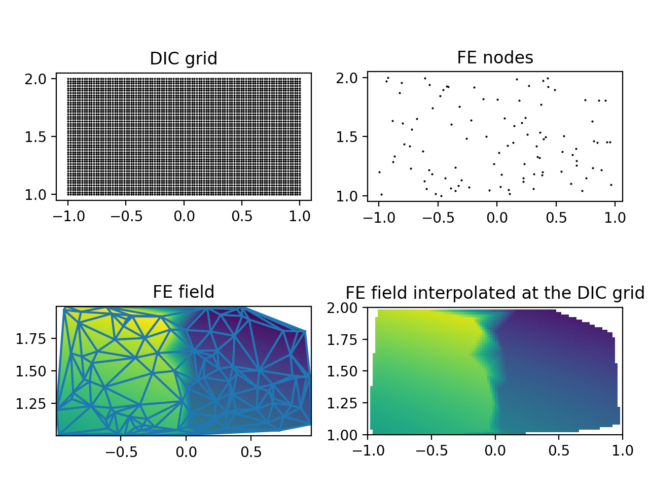
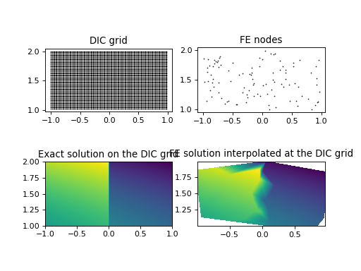